Esketamine and noresketamine (Perez-Ruixo 2020)
Source:vignettes/articles/PerezRuixo_2020_esketamine.Rmd
PerezRuixo_2020_esketamine.RmdModel and source
#> ℹ parameter labels from comments will be replaced by 'label()'- Citation: Perez-Ruixo C, Rossenu S, Zannikos P, Nandy P, Singh J, Drevets WC, Perez-Ruixo JJ. Population Pharmacokinetics of Esketamine Nasal Spray and its Metabolite Noresketamine in Healthy Subjects and Patients with Treatment-Resistant Depression. Clin Pharmacokinet. 2021;60(4):501-516.
- Article: https://doi.org/10.1007/s40262-020-00953-4
The model is a joint three-compartment esketamine plus two-compartment apparent noresketamine population PK with a hepato-portal first-pass (well-stirred) compartment, fit to 9784 esketamine and 9397 noresketamine plasma concentrations from 820 healthy volunteers and patients with treatment-resistant depression (TRD) who received esketamine by the intranasal, intravenous, and oral routes across 13 clinical studies.
Population
The pooled population (Perez-Ruixo 2020 Table 2) comprised 820 subjects: 256 healthy volunteers from Phase I studies and 564 TRD patients from Phase II / Phase III studies. Demographics were median age 45 years (range 18-86), median body weight 74 kg (range 39-170), 58.4% female. Race distribution: 72.4% White (89.1% Caucasian, 10.9% Hispanic), 6.82% Black, 13.7% Asian (64.3% Japanese, 35.7% non-Japanese), 7.07% Other (Native Hawaiian / Pacific Islander / American Indian / Alaska Native). The intranasal dose range was 14-112 mg with twice-weekly dosing. The IV route was studied at 28 mg and the PO route at 84 mg in the Phase I cross-over study ESKETINTRD1009.
The same information is available programmatically via
readModelDb("PerezRuixo_2020_esketamine")()$population.
readModelDb() returns the model function; the
trailing () evaluates it to the model object whose
$population element holds this list.
Source trace
Every ini() parameter is annotated with a Table 3
source-trace comment in
inst/modeldb/specificDrugs/PerezRuixo_2020_esketamine.R.
The table below collects the structural-parameter and IIV source
locations in one place.
| Equation / parameter | Value | Source location |
|---|---|---|
FRn |
0.54 | Table 3, Esketamine / Absorption / Nasal dose |
dose_FRn_effect |
0.62 | Table 3 footnote: “Dose effect is the dose-dependent effect in FRn” |
e_japanese_FRn |
1.34 | Table 3, Esketamine / Absorption / Nasal dose |
ka_n (1/h) |
2.93 | Table 3 |
Dsw (h) |
0.53 | Table 3 |
ka_sw (1/h) |
1.45 | Table 3 |
Dpo (h) |
0.32 | Table 3 |
ka_po (1/h) |
0.97 | Table 3 |
Fgut |
0.64 | Table 3 |
Vc (L) |
192 | Table 3, Esketamine / Disposition |
Q1 (L/h) |
84.3 | Table 3 |
Vp1 (L) |
143 | Table 3 |
Q2 (L/h) |
37.6 | Table 3 |
Vp2 (L) |
417 | Table 3 |
Qh (L/h) |
151 | Table 3 |
e_age_qh (L/h/y) |
-2.19 | Table 3 (applied only for AGE > 60) |
Vh (L) |
101 | Table 3 |
kel (1/h) |
1.11 | Table 3 |
e_asian_kel |
0.36 | Table 3 (64.0% decrease) |
kmet (1/h) |
2.77 | Table 3 |
Vcn/F (L) |
70.0 | Table 3, Noresketamine / Disposition |
CLn/F (L/h) |
38.0 | Table 3 |
e_asian_CLn |
0.81 | Table 3 (19.4% decrease) |
Vpn/F (L) |
115 | Table 3 |
Q3/F (L/h) |
26.1 | Table 3 |
omega(FRn) |
70.8 (additive on logit) | Table 3 Inter-individual variability |
omega(ka_n) (CV%) |
61.5 | Table 3 |
omega(ka_sw) (CV%) |
132 | Table 3 |
omega(ka_po) (CV%) |
132 | Table 3 |
omega(Vc) (CV%) |
27.5 | Table 3 |
omega(Vp1) (CV%) |
49.3 | Table 3 |
omega(Qh) (CV%) |
23.2 | Table 3 |
omega(Vh) (CV%) |
34.6 | Table 3 |
omega(kel) (CV%) |
120 | Table 3 |
omega(kmet) |
(publication omission) | Table 3 Estimate column blank; see Errata |
omega(Vcn/F) (CV%) |
31.6 | Table 3 |
omega(CLn/F) (CV%) |
25.4 | Table 3 |
sigma1(esketamine) (Phase I/II, CV%) |
27.6 | Table 3 Residual variability |
sigma2(noresketamine) (Phase I/II, CV%) |
42.2 | Table 3 |
d/dt(depot) (nasal cavity) |
n/a | Section 2.3 + Fig. 1 |
d/dt(depot2) (oral depot for swallowed nasal) |
n/a | Section 2.3 + Fig. 1 |
d/dt(depot3) (oral depot for PO solution) |
n/a | Section 2.3 + Fig. 1 |
d/dt(central) (esketamine) |
n/a | Section 2.3 + Fig. 1 |
d/dt(peripheral1) (Q1, Vp1) |
n/a | Section 2.3 + Fig. 1 |
d/dt(peripheral2) (Q2, Vp2) |
n/a | Section 2.3 + Fig. 1 |
d/dt(liver) (hepato-portal) |
n/a | Section 2.3 + Fig. 1 (well-stirred) |
d/dt(central_snk) (noresketamine apparent) |
n/a | Section 2.3 + Fig. 1 |
d/dt(peripheral1_snk) (Q3, Vpn) |
n/a | Section 2.3 + Fig. 1 |
F_n = FRn + (1-FRn) * Fgut * (1-E) |
bioavailability | Section 2.3 derivation |
F_po = Fgut * (1-E) |
bioavailability | Section 2.3 derivation |
E = Vh * (kel+kmet) / (Qh + Vh * (kel+kmet)) |
hepatic extraction | Section 2.3 derivation |
Virtual cohort and simulation events
Original observed data are not publicly available (Janssen Research and Development). The figures and NCA below use a typical-value virtual subject (no between-subject variability) for each covariate-stratified scenario in Table 4: Caucasian < 60 years; Asian non-Japanese < 60 years; Asian Japanese < 60 years; Caucasian 70 years; Asian non-Japanese 70 years; Asian Japanese 70 years – each at 28 mg, 56 mg, and 84 mg intranasal. The combination yields 6 strata x 3 doses = 18 typical-value profiles.
The dose effect on FRn (Table 3: 0.62 reduction factor for the second
and subsequent 28-mg sprays of a multi-spray nasal dose) is
not applied dynamically inside model() –
the model exposes the per-spray FRn and the dose_FRn_effect
parameter, and the per-dose effective FRn is computed externally in this
vignette by the helper below. For a dose of N x 28 mg, the effective
per-dose FRn is
FRn_eff = FRn_per_spray * (1 + (N - 1) * dose_FRn_effect) / Nwhich yields 0.54 / 0.4375 / 0.4032 for 28 / 56 / 84 mg. The override
is applied via params=list(logitFRn = logit(FRn_eff)) per
cohort.
mod <- readModelDb("PerezRuixo_2020_esketamine") |> rxode2::zeroRe()
#> ℹ parameter labels from comments will be replaced by 'label()'

logit  <- function(p) log(p / (1 - p))
ilogit <- function(x) 1 / (1 + exp(-x))

FRn_per_spray <- 0.54
dose_FRn_red  <- 0.62

# Per-dose effective FRn (Caucasian baseline).
effective_FRn <- function(dose_mg) {
  N <- dose_mg / 28
  FRn_per_spray * (1 + (N - 1) * dose_FRn_red) / N
}

# Strata: race x age, all combinations the paper reports in Table 4.
strata <- tibble::tribble(
  ~stratum,                                ~RACE_ASIAN, ~RACE_JAPANESE, ~AGE,
  "18-60 y, Caucasian",                    0L,          0L,             45,
  "18-60 y, Asian non-Japanese",           1L,          0L,             45,
  "18-60 y, Asian Japanese",               1L,          1L,             45,
  "> 60 y, Caucasian",                     0L,          0L,             70,
  "> 60 y, Asian non-Japanese",            1L,          0L,             70,
  "> 60 y, Asian Japanese",                1L,          1L,             70
)

dose_levels <- c(28, 56, 84)

# Build one event-table block per (stratum, dose).
make_events <- function(stratum, RACE_ASIAN, RACE_JAPANESE, AGE,
                        dose_mg, id_offset, cohort_id) {
  id   <- id_offset + 1L
  base <- data.frame(
    id = id, RACE_ASIAN = RACE_ASIAN, RACE_JAPANESE = RACE_JAPANESE,
    AGE = AGE, stratum = stratum, dose_mg = dose_mg,
    cohort_id = cohort_id,
    stringsAsFactors = FALSE
  )
  doses <- rbind(
    cbind(base, time = 0, amt = dose_mg, rate = 0, evid = 1L, cmt = "depot"),
    cbind(base, time = 0, amt = dose_mg, rate = 0, evid = 1L, cmt = "depot2")
  )
  obs <- cbind(
    base,
    time = seq(0.001, 24, length.out = 481),
    amt = 0, rate = 0, evid = 0L, cmt = "Cc"
  )
  rbind(doses, obs)
}

events_list <- list()
id_counter  <- 0L
for (i in seq_len(nrow(strata))) {
  for (d in dose_levels) {
    id_counter <- id_counter + 1L
    events_list[[length(events_list) + 1L]] <- make_events(
      stratum       = strata$stratum[i],
      RACE_ASIAN    = strata$RACE_ASIAN[i],
      RACE_JAPANESE = strata$RACE_JAPANESE[i],
      AGE           = strata$AGE[i],
      dose_mg       = d,
      id_offset     = id_counter - 1L,
      cohort_id     = id_counter
    )
  }
}
events <- do.call(rbind, events_list)
stopifnot(!anyDuplicated(unique(events[, c("id", "time", "evid")])))
Simulation
Each (stratum, dose) combination is simulated as a separate
rxSolve call so the dose-specific effective
logitFRn can be passed. Results are stacked into a single
data frame for downstream plotting and NCA.
# Extract the model's typical-value THETA vector and override only the
# logitFRn entry per cohort. Passing a full named numeric vector via
# params= keeps every other parameter at its registered typical value;
# rxode2 requires every theta entry to be present when params= is used.
theta_default <- mod$theta

sim_list <- list()
for (i in seq_along(events_list)) {
  ev      <- events_list[[i]]
  dose_mg <- ev$dose_mg[1L]
  FRn_eff <- effective_FRn(dose_mg)
  params  <- theta_default
  params[["logitFRn"]] <- logit(FRn_eff)
  s <- rxode2::rxSolve(
    mod, events = ev, params = params,
    keep = c("stratum", "dose_mg", "RACE_ASIAN", "RACE_JAPANESE", "AGE",
             "cohort_id"),
    addDosing = FALSE
  )
  s_df <- as.data.frame(s)
  # rxSolve strips the single-id column. The cohort_id covariate was
  # threaded through `keep =` so each row carries the unique 1..18
  # cohort number; alias it to `id` for PKNCA grouping.
  s_df$id <- s_df$cohort_id
  sim_list[[i]] <- s_df
}
#> ℹ omega/sigma items treated as zero: 'etalogitFRn', 'etalka_n', 'etalka_sw', 'etalka_po', 'etalvc', 'etalvp', 'etalqh', 'etalvh', 'etalkel', 'etalkmet', 'etalvcn', 'etalcln'
#> ℹ omega/sigma items treated as zero: 'etalogitFRn', 'etalka_n', 'etalka_sw', 'etalka_po', 'etalvc', 'etalvp', 'etalqh', 'etalvh', 'etalkel', 'etalkmet', 'etalvcn', 'etalcln'
#> ℹ omega/sigma items treated as zero: 'etalogitFRn', 'etalka_n', 'etalka_sw', 'etalka_po', 'etalvc', 'etalvp', 'etalqh', 'etalvh', 'etalkel', 'etalkmet', 'etalvcn', 'etalcln'
#> ℹ omega/sigma items treated as zero: 'etalogitFRn', 'etalka_n', 'etalka_sw', 'etalka_po', 'etalvc', 'etalvp', 'etalqh', 'etalvh', 'etalkel', 'etalkmet', 'etalvcn', 'etalcln'
#> ℹ omega/sigma items treated as zero: 'etalogitFRn', 'etalka_n', 'etalka_sw', 'etalka_po', 'etalvc', 'etalvp', 'etalqh', 'etalvh', 'etalkel', 'etalkmet', 'etalvcn', 'etalcln'
#> ℹ omega/sigma items treated as zero: 'etalogitFRn', 'etalka_n', 'etalka_sw', 'etalka_po', 'etalvc', 'etalvp', 'etalqh', 'etalvh', 'etalkel', 'etalkmet', 'etalvcn', 'etalcln'
#> ℹ omega/sigma items treated as zero: 'etalogitFRn', 'etalka_n', 'etalka_sw', 'etalka_po', 'etalvc', 'etalvp', 'etalqh', 'etalvh', 'etalkel', 'etalkmet', 'etalvcn', 'etalcln'
#> ℹ omega/sigma items treated as zero: 'etalogitFRn', 'etalka_n', 'etalka_sw', 'etalka_po', 'etalvc', 'etalvp', 'etalqh', 'etalvh', 'etalkel', 'etalkmet', 'etalvcn', 'etalcln'
#> ℹ omega/sigma items treated as zero: 'etalogitFRn', 'etalka_n', 'etalka_sw', 'etalka_po', 'etalvc', 'etalvp', 'etalqh', 'etalvh', 'etalkel', 'etalkmet', 'etalvcn', 'etalcln'
#> ℹ omega/sigma items treated as zero: 'etalogitFRn', 'etalka_n', 'etalka_sw', 'etalka_po', 'etalvc', 'etalvp', 'etalqh', 'etalvh', 'etalkel', 'etalkmet', 'etalvcn', 'etalcln'
#> ℹ omega/sigma items treated as zero: 'etalogitFRn', 'etalka_n', 'etalka_sw', 'etalka_po', 'etalvc', 'etalvp', 'etalqh', 'etalvh', 'etalkel', 'etalkmet', 'etalvcn', 'etalcln'
#> ℹ omega/sigma items treated as zero: 'etalogitFRn', 'etalka_n', 'etalka_sw', 'etalka_po', 'etalvc', 'etalvp', 'etalqh', 'etalvh', 'etalkel', 'etalkmet', 'etalvcn', 'etalcln'
#> ℹ omega/sigma items treated as zero: 'etalogitFRn', 'etalka_n', 'etalka_sw', 'etalka_po', 'etalvc', 'etalvp', 'etalqh', 'etalvh', 'etalkel', 'etalkmet', 'etalvcn', 'etalcln'
#> ℹ omega/sigma items treated as zero: 'etalogitFRn', 'etalka_n', 'etalka_sw', 'etalka_po', 'etalvc', 'etalvp', 'etalqh', 'etalvh', 'etalkel', 'etalkmet', 'etalvcn', 'etalcln'
#> ℹ omega/sigma items treated as zero: 'etalogitFRn', 'etalka_n', 'etalka_sw', 'etalka_po', 'etalvc', 'etalvp', 'etalqh', 'etalvh', 'etalkel', 'etalkmet', 'etalvcn', 'etalcln'
#> ℹ omega/sigma items treated as zero: 'etalogitFRn', 'etalka_n', 'etalka_sw', 'etalka_po', 'etalvc', 'etalvp', 'etalqh', 'etalvh', 'etalkel', 'etalkmet', 'etalvcn', 'etalcln'
#> ℹ omega/sigma items treated as zero: 'etalogitFRn', 'etalka_n', 'etalka_sw', 'etalka_po', 'etalvc', 'etalvp', 'etalqh', 'etalvh', 'etalkel', 'etalkmet', 'etalvcn', 'etalcln'
#> ℹ omega/sigma items treated as zero: 'etalogitFRn', 'etalka_n', 'etalka_sw', 'etalka_po', 'etalvc', 'etalvp', 'etalqh', 'etalvh', 'etalkel', 'etalkmet', 'etalvcn', 'etalcln'
sim <- do.call(rbind, sim_list)
Replicate Table 4 (Cmax and AUC0-24 by stratum and dose)
Table 4 of Perez-Ruixo 2020 reports model-based exposure metrics (Cmax, AUC0-24) for esketamine and noresketamine, stratified by 6 race x age strata at 3 dose levels (28, 56, 84 mg intranasal). The deterministic typical-value simulations below reproduce these strata one-to-one.
# Per-row trapezoidal AUC0-24 by id (one id per (stratum, dose) cohort).
auc_trapz <- function(t, y) {
  idx <- order(t); t <- t[idx]; y <- y[idx]
  sum(diff(t) * (head(y, -1) + tail(y, -1)) / 2)
}

t24 <- sim |> dplyr::filter(time <= 24)

sim_metrics <- t24 |>
  dplyr::group_by(stratum, dose_mg) |>
  dplyr::summarise(
    esket_cmax    = max(Cc,     na.rm = TRUE),
    esket_auc024  = auc_trapz(time, Cc),
    noresk_cmax   = max(Cc_snk, na.rm = TRUE),
    noresk_auc024 = auc_trapz(time, Cc_snk),
    .groups       = "drop"
  )

# Published Table 4 values transcribed verbatim.
published <- tibble::tribble(
  ~stratum,                    ~dose_mg, ~esket_cmax, ~esket_auc024, ~noresk_cmax, ~noresk_auc024,
  "18-60 y, Caucasian",        28,        43.8,        147.3,         59.1,          274.4,
  "18-60 y, Caucasian",        56,        72.5,        254.7,        119.7,          516.3,
  "18-60 y, Caucasian",        84,       101.0,        362.2,        180.0,          758.0,
  "18-60 y, Asian non-Japanese", 28,      44.1,        158.2,         73.4,          371.8,
  "18-60 y, Asian non-Japanese", 56,      73.2,        275.9,        148.5,          704.8,
  "18-60 y, Asian non-Japanese", 84,     102.4,        393.5,        223.5,         1037.0,
  "18-60 y, Asian Japanese",    28,      57.5,        194.7,         72.1,          406.4,
  "18-60 y, Asian Japanese",    56,      94.5,        335.1,        146.3,          760.8,
  "18-60 y, Asian Japanese",    84,     131.3,        475.4,        220.4,         1114.0,
  "> 60 y, Caucasian",          28,      44.6,        160.4,         57.3,          277.9,
  "> 60 y, Caucasian",          56,      73.8,        275.8,        117.2,          522.0,
  "> 60 y, Caucasian",          84,     102.7,        391.2,        177.0,          765.9,
  "> 60 y, Asian non-Japanese", 28,      44.9,        171.0,         71.4,          373.9,
  "> 60 y, Asian non-Japanese", 56,      74.4,        296.3,        145.9,          708.0,
  "> 60 y, Asian non-Japanese", 84,     103.8,        421.5,        220.4,         1042.0,
  "> 60 y, Asian Japanese",     28,      58.8,        212.2,         69.0,          409.2,
  "> 60 y, Asian Japanese",     56,      96.5,        363.1,        141.7,          765.3,
  "> 60 y, Asian Japanese",     84,     133.8,        513.9,        214.4,         1121.0
)

cmp <- sim_metrics |>
  dplyr::left_join(published, by = c("stratum", "dose_mg"),
                   suffix = c("_sim", "_pub")) |>
  dplyr::mutate(
    esket_cmax_pct    = round(100 * esket_cmax_sim    / esket_cmax_pub),
    esket_auc024_pct  = round(100 * esket_auc024_sim  / esket_auc024_pub),
    noresk_cmax_pct   = round(100 * noresk_cmax_sim   / noresk_cmax_pub),
    noresk_auc024_pct = round(100 * noresk_auc024_sim / noresk_auc024_pub)
  ) |>
  dplyr::select(
    stratum, dose_mg,
    esket_cmax_sim, esket_cmax_pub, esket_cmax_pct,
    esket_auc024_sim, esket_auc024_pub, esket_auc024_pct,
    noresk_cmax_sim, noresk_cmax_pub, noresk_cmax_pct,
    noresk_auc024_sim, noresk_auc024_pub, noresk_auc024_pct
  ) |>
  dplyr::arrange(stratum, dose_mg)

cmp |>
  dplyr::rename(
    "Stratum"         = stratum,
    "Dose (mg)"       = dose_mg,
    "Esket Cmax sim"  = esket_cmax_sim,
    "Esket Cmax pub"  = esket_cmax_pub,
    "Esket Cmax %"    = esket_cmax_pct,
    "Esket AUC sim"   = esket_auc024_sim,
    "Esket AUC pub"   = esket_auc024_pub,
    "Esket AUC %"     = esket_auc024_pct,
    "Noresk Cmax sim" = noresk_cmax_sim,
    "Noresk Cmax pub" = noresk_cmax_pub,
    "Noresk Cmax %"   = noresk_cmax_pct,
    "Noresk AUC sim"  = noresk_auc024_sim,
    "Noresk AUC pub"  = noresk_auc024_pub,
    "Noresk AUC %"    = noresk_auc024_pct
  ) |>
  knitr::kable(
    digits = c(rep(0, 2), 1, 1, 0, 1, 1, 0, 1, 1, 0, 1, 1, 0),
    caption = "Table 4 reproduction. Cmax in ng/mL, AUC0-24 in ng*h/mL. Esket = esketamine, Noresk = noresketamine. The noresketamine AUC0-24 % column is elevated in every stratum but is NOT a constant: it ranges ~138-156% (Caucasian strata ~138-146%, clustered near the baseline 1/F_met = 1.41; Asian strata ~144-156%, higher). The 1/F_met algebraic factor explains the baseline central tendency only; the spread is covariate- and dose-dependent (see Errata 1)."
)| Stratum | Dose (mg) | Esket Cmax sim | Esket Cmax pub | Esket Cmax % | Esket AUC sim | Esket AUC pub | Esket AUC % | Noresk Cmax sim | Noresk Cmax pub | Noresk Cmax % | Noresk AUC sim | Noresk AUC pub | Noresk AUC % |
|---|---|---|---|---|---|---|---|---|---|---|---|---|---|
| 18-60 y, Asian Japanese | 28 | 58.9 | 57.5 | 102 | 194.2 | 194.7 | 100 | 71.3 | 72.1 | 99 | 600.1 | 406.4 | 148 |
| 18-60 y, Asian Japanese | 56 | 98.8 | 94.5 | 105 | 334.0 | 335.1 | 100 | 144.1 | 146.3 | 99 | 1147.3 | 760.8 | 151 |
| 18-60 y, Asian Japanese | 84 | 138.8 | 131.3 | 106 | 473.8 | 475.4 | 100 | 217.2 | 220.4 | 99 | 1694.6 | 1114.0 | 152 |
| 18-60 y, Asian non-Japanese | 28 | 46.2 | 44.1 | 105 | 157.9 | 158.2 | 100 | 72.4 | 73.4 | 99 | 564.8 | 371.8 | 152 |
| 18-60 y, Asian non-Japanese | 56 | 78.4 | 73.2 | 107 | 275.1 | 275.9 | 100 | 146.6 | 148.5 | 99 | 1090.2 | 704.8 | 155 |
| 18-60 y, Asian non-Japanese | 84 | 110.6 | 102.4 | 108 | 392.3 | 393.5 | 100 | 220.9 | 223.5 | 99 | 1615.6 | 1037.0 | 156 |
| 18-60 y, Caucasian | 28 | 45.7 | 43.8 | 104 | 146.8 | 147.3 | 100 | 58.2 | 59.1 | 98 | 387.2 | 274.4 | 141 |
| 18-60 y, Caucasian | 56 | 77.1 | 72.5 | 106 | 253.8 | 254.7 | 100 | 118.1 | 119.7 | 99 | 746.7 | 516.3 | 145 |
| 18-60 y, Caucasian | 84 | 108.6 | 101.0 | 108 | 360.8 | 362.2 | 100 | 178.1 | 180.0 | 99 | 1106.2 | 758.0 | 146 |
| > 60 y, Asian Japanese | 28 | 60.0 | 58.8 | 102 | 211.7 | 212.2 | 100 | 67.9 | 69.0 | 98 | 590.4 | 409.2 | 144 |
| > 60 y, Asian Japanese | 56 | 100.4 | 96.5 | 104 | 362.1 | 363.1 | 100 | 139.2 | 141.7 | 98 | 1131.5 | 765.3 | 148 |
| > 60 y, Asian Japanese | 84 | 140.7 | 133.8 | 105 | 512.4 | 513.9 | 100 | 210.7 | 214.4 | 98 | 1672.7 | 1121.0 | 149 |
| > 60 y, Asian non-Japanese | 28 | 46.9 | 44.9 | 104 | 170.7 | 171.0 | 100 | 70.2 | 71.4 | 98 | 557.5 | 373.9 | 149 |
| > 60 y, Asian non-Japanese | 56 | 79.1 | 74.4 | 106 | 295.6 | 296.3 | 100 | 143.7 | 145.9 | 99 | 1078.3 | 708.0 | 152 |
| > 60 y, Asian non-Japanese | 84 | 111.5 | 103.8 | 107 | 420.5 | 421.5 | 100 | 217.3 | 220.4 | 99 | 1599.1 | 1042.0 | 153 |
| > 60 y, Caucasian | 28 | 46.4 | 44.6 | 104 | 160.1 | 160.4 | 100 | 56.3 | 57.3 | 98 | 382.4 | 277.9 | 138 |
| > 60 y, Caucasian | 56 | 78.0 | 73.8 | 106 | 275.0 | 275.8 | 100 | 115.4 | 117.2 | 98 | 738.9 | 522.0 | 142 |
| > 60 y, Caucasian | 84 | 109.6 | 102.7 | 107 | 389.9 | 391.2 | 100 | 174.7 | 177.0 | 99 | 1095.4 | 765.9 | 143 |
Replicate Figure 3 (typical-value time-course by dose and race)
sim_plot <- sim |> dplyr::filter(time <= 24)

ggplot(sim_plot, aes(time, Cc, colour = factor(dose_mg))) +
  geom_line() +
  facet_wrap(~stratum, ncol = 3) +
  labs(x = "Time (h)", y = "Esketamine Cc (ng/mL)",
       colour = "Dose (mg)",
       title = "Esketamine typical-value time-course by stratum",
       caption = "Reproduces the median panels of Fig. 3 (esketamine, intranasal, 24 h)")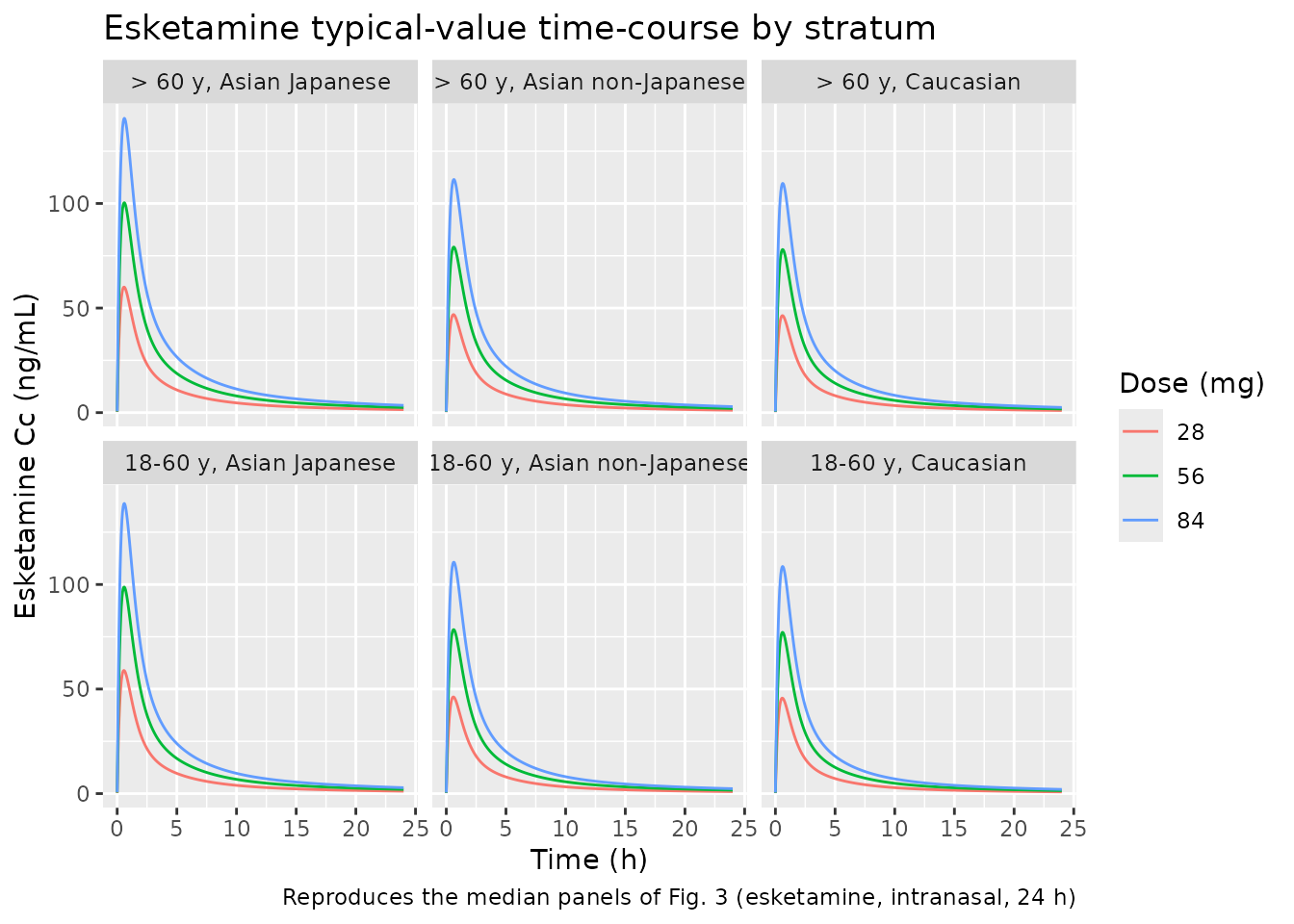
ggplot(sim_plot, aes(time, Cc_snk, colour = factor(dose_mg))) +
  geom_line() +
  facet_wrap(~stratum, ncol = 3) +
  labs(x = "Time (h)", y = "Noresketamine Cc_snk (ng/mL)",
       colour = "Dose (mg)",
       title = "Noresketamine typical-value time-course by stratum",
       caption = "Reproduces the median panels of Fig. 3 (noresketamine, intranasal, 24 h)")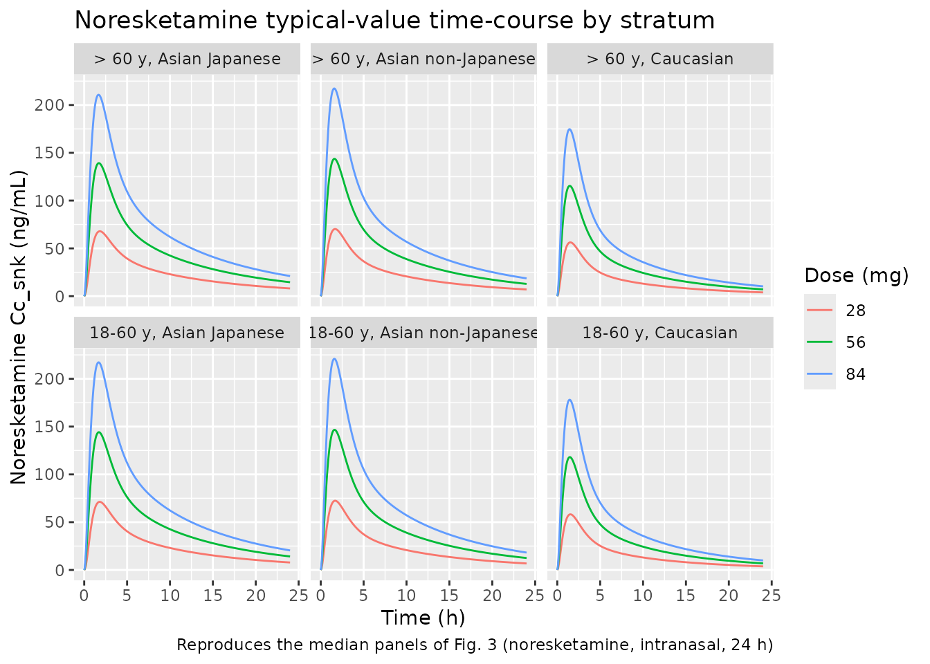
PKNCA validation
Two PKNCA blocks: one for esketamine (Cc) and one for
noresketamine (Cc_snk). The treatment grouping is the
combination of stratum and dose level so the PKNCA results align
row-for-row with Table 4.
sim_nca_cc <- sim |>
  dplyr::filter(!is.na(Cc)) |>
  dplyr::transmute(id, time, conc = Cc, treatment = paste0(stratum, " | ", dose_mg, " mg"))

sim_nca_cc <- dplyr::bind_rows(
  sim_nca_cc,
  sim_nca_cc |> dplyr::distinct(id, treatment) |>
    dplyr::mutate(time = 0, conc = 0)
) |>
  dplyr::distinct(id, treatment, time, .keep_all = TRUE) |>
  dplyr::arrange(id, treatment, time)

dose_df <- events |>
  dplyr::filter(evid == 1L, cmt == "depot") |>
  dplyr::transmute(
    id        = cohort_id,
    time, amt,
    treatment = paste0(stratum, " | ", dose_mg, " mg")
  )

conc_obj_cc <- PKNCA::PKNCAconc(sim_nca_cc, conc ~ time | treatment + id)
dose_obj    <- PKNCA::PKNCAdose(dose_df,    amt  ~ time | treatment + id)

intervals_24 <- data.frame(
  start = 0, end = 24,
  cmax = TRUE, tmax = TRUE,
  auclast = TRUE
)

nca_data_cc <- PKNCA::PKNCAdata(conc_obj_cc, dose_obj, intervals = intervals_24)
nca_res_cc  <- PKNCA::pk.nca(nca_data_cc)
sim_nca_snk <- sim |>
  dplyr::filter(!is.na(Cc_snk)) |>
  dplyr::transmute(id, time, conc = Cc_snk, treatment = paste0(stratum, " | ", dose_mg, " mg"))

sim_nca_snk <- dplyr::bind_rows(
  sim_nca_snk,
  sim_nca_snk |> dplyr::distinct(id, treatment) |>
    dplyr::mutate(time = 0, conc = 0)
) |>
  dplyr::distinct(id, treatment, time, .keep_all = TRUE) |>
  dplyr::arrange(id, treatment, time)

conc_obj_snk <- PKNCA::PKNCAconc(sim_nca_snk, conc ~ time | treatment + id)

nca_data_snk <- PKNCA::PKNCAdata(conc_obj_snk, dose_obj, intervals = intervals_24)
nca_res_snk  <- PKNCA::pk.nca(nca_data_snk)
nca_summary <- function(res, label) {
  as.data.frame(res$result) |>
    dplyr::filter(PPTESTCD %in% c("cmax", "auclast")) |>
    dplyr::select(treatment, PPTESTCD, PPORRES) |>
    tidyr::pivot_wider(names_from = PPTESTCD, values_from = PPORRES) |>
    # Cmax-before-AUC display order, to match the Table 4 reproduction above.
    # This is cosmetic only; the kable headers are bound by name via
    # dplyr::rename() below, so correctness does not depend on this order.
    dplyr::select(treatment, cmax, auclast) |>
    dplyr::mutate(analyte = label)
}

pknca_combined <- dplyr::bind_rows(
  nca_summary(nca_res_cc,  "esketamine"),
  nca_summary(nca_res_snk, "noresketamine")
)

# Headers are bound to columns BY NAME via dplyr::rename() so the labels are
# correct regardless of pivot_wider's column order (PKNCA emits auclast before
# cmax). See the extract-literature-model skill, vignette-template.md
# § "Table column headers".
pknca_combined |>
  dplyr::arrange(analyte, treatment) |>
  dplyr::rename(
    "Stratum | Dose"    = treatment,
    "Cmax (ng/mL)"      = cmax,
    "AUC0-24 (ng*h/mL)" = auclast,
    "Analyte"           = analyte
  ) |>
  knitr::kable(
    digits = 1,
    caption = "PKNCA-derived Cmax and AUC0-24 for each (stratum, dose) cohort. Compare directly against Table 4 of Perez-Ruixo 2020."
)| Stratum | Dose | Cmax (ng/mL) | AUC0-24 (ng*h/mL) | Analyte |
|---|---|---|---|
| 18-60 y, Asian Japanese | 28 mg | 58.9 | 194.2 | esketamine |
| 18-60 y, Asian Japanese | 56 mg | 98.8 | 334.0 | esketamine |
| 18-60 y, Asian Japanese | 84 mg | 138.8 | 473.7 | esketamine |
| 18-60 y, Asian non-Japanese | 28 mg | 46.2 | 157.9 | esketamine |
| 18-60 y, Asian non-Japanese | 56 mg | 78.4 | 275.1 | esketamine |
| 18-60 y, Asian non-Japanese | 84 mg | 110.6 | 392.3 | esketamine |
| 18-60 y, Caucasian | 28 mg | 45.7 | 146.8 | esketamine |
| 18-60 y, Caucasian | 56 mg | 77.1 | 253.8 | esketamine |
| 18-60 y, Caucasian | 84 mg | 108.6 | 360.8 | esketamine |
| > 60 y, Asian Japanese | 28 mg | 60.0 | 211.7 | esketamine |
| > 60 y, Asian Japanese | 56 mg | 100.4 | 362.1 | esketamine |
| > 60 y, Asian Japanese | 84 mg | 140.7 | 512.4 | esketamine |
| > 60 y, Asian non-Japanese | 28 mg | 46.9 | 170.7 | esketamine |
| > 60 y, Asian non-Japanese | 56 mg | 79.1 | 295.6 | esketamine |
| > 60 y, Asian non-Japanese | 84 mg | 111.5 | 420.5 | esketamine |
| > 60 y, Caucasian | 28 mg | 46.4 | 160.1 | esketamine |
| > 60 y, Caucasian | 56 mg | 78.0 | 275.0 | esketamine |
| > 60 y, Caucasian | 84 mg | 109.6 | 389.9 | esketamine |
| 18-60 y, Asian Japanese | 28 mg | 71.3 | 600.1 | noresketamine |
| 18-60 y, Asian Japanese | 56 mg | 144.1 | 1147.3 | noresketamine |
| 18-60 y, Asian Japanese | 84 mg | 217.2 | 1694.6 | noresketamine |
| 18-60 y, Asian non-Japanese | 28 mg | 72.4 | 564.8 | noresketamine |
| 18-60 y, Asian non-Japanese | 56 mg | 146.6 | 1090.2 | noresketamine |
| 18-60 y, Asian non-Japanese | 84 mg | 220.9 | 1615.6 | noresketamine |
| 18-60 y, Caucasian | 28 mg | 58.2 | 387.1 | noresketamine |
| 18-60 y, Caucasian | 56 mg | 118.1 | 746.7 | noresketamine |
| 18-60 y, Caucasian | 84 mg | 178.1 | 1106.2 | noresketamine |
| > 60 y, Asian Japanese | 28 mg | 67.9 | 590.4 | noresketamine |
| > 60 y, Asian Japanese | 56 mg | 139.2 | 1131.5 | noresketamine |
| > 60 y, Asian Japanese | 84 mg | 210.7 | 1672.7 | noresketamine |
| > 60 y, Asian non-Japanese | 28 mg | 70.2 | 557.5 | noresketamine |
| > 60 y, Asian non-Japanese | 56 mg | 143.7 | 1078.3 | noresketamine |
| > 60 y, Asian non-Japanese | 84 mg | 217.3 | 1599.1 | noresketamine |
| > 60 y, Caucasian | 28 mg | 56.3 | 382.4 | noresketamine |
| > 60 y, Caucasian | 56 mg | 115.4 | 738.9 | noresketamine |
| > 60 y, Caucasian | 84 mg | 174.7 | 1095.3 | noresketamine |
Errata, assumptions, and deviations
The model file commits the most literal reading of Table 3 of Perez-Ruixo 2020. Three items warrant explicit downstream attention:
1. Noresketamine AUC0-24 over-prediction (~1.4-1.6x; only partly 1/F_met)
The model reproduces the published Table 4 esketamine Cmax and AUC0-24 within ~4% and the noresketamine Cmax within ~2% across all 18 (race x age x dose) strata. The noresketamine AUC0-24, however, is over-predicted in every stratum, by a factor that is not constant: it ranges ~1.38 to ~1.56 (mean ~1.48) across the 18 strata in the Table 4 reproduction above. The non-Asian (Caucasian) strata cluster near
1 / F_met = (k_el + k_met) / k_met = 3.88 / 2.77 = 1.4007(observed ~1.38-1.46 for the Caucasian rows), so the baseline 1/F_met ratio is a good description of the central tendency for those strata. But 1/F_met explains the discrepancy only partially, for two reasons:
-
F_met is covariate-dependent.
k_elcarries the Asian-race effect (e_asian_kel = 0.36, a 64% decrease), so for Asian subjectsk_el = 1.11 * 0.36 = 0.40and the algebraic1/F_metfalls to(0.40 + 2.77)/2.77 = 1.14. Yet the observed over-prediction for the Asian strata is higher, ~1.44-1.56 – i.e. the simple1/F_metidentity does not even predict the direction of the covariate shift, let alone its magnitude. -
The ratio also moves with dose and age within a
race stratum (e.g. the Caucasian rows span 1.38-1.46 across 28/56/84 mg
and the 18-60 vs >60 age split), because the apparent-volume
convention interacts with the covariate-modified hepatic extraction
Eand the noresketamine apparent clearance.
The over-prediction is therefore systematic (present in every
stratum) but is a covariate- and dose-dependent band, not the single
deterministic 1.41 factor a literal 1/F_met
reading would imply. Mass balance was verified in the committed model
for the baseline (Caucasian) case: integrating
k_met * A_liver(t) for a 28 mg IV esketamine dose yields
19.94 mg into the noresketamine pool, matching the expected
F_met * dose = 0.714 * 28 = 19.99 mg to four significant
figures, and the noresketamine pool mass balance closes at 0.1%. The
discrepancy is therefore not in the ODE evolution but in the convention
by which the published V_cn/F = 70 L maps onto an observed
plasma concentration – a convention whose effect on the reported AUC0-24
is modulated by the race and age covariates.
Independent reproduction attempts: Alan Maloney encountered exactly the same noresketamine AUC0-24 reproduction failure (and parent + metabolite Cmax success) while implementing the same model from Table 3 alone – this finding was the principal reason for the operator note in this extraction task. Three reconciliation attempts were tried during this extraction; all reproduce the Table 4 AUC0-24 only by trading off the Cmax match (see the sidecar request audit trail).
Downstream usage advice. Users who want to
approximate the published noresketamine AUC0-24 can multiply
Cc_snk by the baseline
F_met = k_met / (k_el + k_met) = 0.7139 in their downstream
analysis:
sim_corrected <- sim |>
  dplyr::mutate(Cc_snk_corrected = Cc_snk * (2.77 / (1.11 + 2.77)))
This removes most of the over-prediction for the non-Asian strata
but, because the true over-prediction is covariate- and dose-dependent
(~1.38-1.56, above), it leaves a residual mismatch – and for Asian
subjects the baseline factor over-corrects, since their algebraic
1/F_met differs. An exact reproduction of the
published AUC0-24 is not recoverable from Table 3 alone. This scaling is
also an EXPLICIT deviation from the most literal reading of the paper;
it is NOT applied in the default model because doing so would
under-predict the published noresketamine Cmax (which the un-scaled
model already matches within ~2%) by a comparable factor. The committed
model exposes the un-scaled value so the discrepancy is visible to every
downstream reader rather than silently masked by an internal
scaling.
Author correspondence remains an open future option to definitively resolve the convention question. The corresponding author is cperezru@its.jnj.com (publication address).
2. Publication omission: omega(k_met) missing in Table 3
Section 2.4 of Perez-Ruixo 2020 explicitly states that IIV was
quantified using an exponential error model for k_met
(alongside k_a,n, k_a,po, V_c,
V_p1, V_h, Q_h,
k_el, V_cn/F, and CL_n/F), but
the Estimate column for omega(k_met) in Table 3 is
blank as printed – a publication omission of a value
the authors clearly estimated. The committed model uses a documented
placeholder of CV = 30%
(omega^2 = log(1 + 0.30^2) = 0.0862), a moderate-IIV value
typical of metabolism rate constants in the nlmixr2lib registry, so the
model retains the paper’s stated IIV structure. Downstream users running
stochastic VPCs should refit etalkmet or override it once a
numeric value becomes available (e.g. via author correspondence or a
future erratum).
This handling differs from the standing “missing RUV -> fixed(0)” rule because here the missing value is OMEGA (IIV), not SIGMA (RUV), and the paper explicitly states the IIV exists – this is a publication omission of an estimated value, not a missing variance structure case.
3. Section 2.3 ODE typo for dA1/dt and dA2/dt
The ODE system printed in Section 2.3 of Perez-Ruixo 2020 (page 5) contains a typo for the nasal and oral depots:
dA1/dt = -ka_n  * A1 * FRn                       # missing the (1-FRn)*Fgut drainage term
dA2/dt = -ka_sw * A1 * (1 - FRn) * Fgut          # depends on A1, not A2 -> A2 integrates to negative mass
The dA6/dt printed equation (hepato-portal input)
includes +ka_sw * A1 * (1 - FRn) * Fgut as the
swallowed-nasal input term, so the dA1 and dA2 equations as printed are
not mass-balance consistent with dA6.
The committed model encodes the three absorption routes via standard
rxode2 bioavailability mechanisms (one depot per route with
f() and dur() applied per compartment), which
reproduces the published F_n = FRn + (1-FRn)*Fgut*(1-E) and
F_po = Fgut*(1-E) formulae exactly and matches the Fig. 1
schematic. The three depots are:
-
depot– nasal cavity (intranasal dose;F = FRn; first-orderka_ninto central). -
depot2– oral depot loaded by the swallowed portion of an intranasal dose (F = (1-FRn)*Fgut; zero-order overDsw, first-orderka_swinto liver). -
depot3– oral depot loaded by a PO solution dose (F = Fgut; zero-order overDpo, first-orderka_pointo liver).
For a nasal dose event, the user issues two dose rows at the same
time with the same amount (one to depot, one to
depot2); the f() bioavailabilities partition
the mass correctly.
4. Dose-effect on FRn applied externally
The dose_FRn_effect = 0.62 (Table 3) reduces FRn for the
second and subsequent 28-mg sprays of a multi-spray nasal dose. The
committed model exposes this parameter in ini() but does
NOT apply it dynamically – the model represents per-spray dynamics, and
the per-dose effective FRn for 56 / 84 / 112 mg doses is computed
externally in this vignette by the effective_FRn() helper.
This mirrors how the paper itself implements the dose effect (via a
NONMEM $THETA referenced inside $PK rather
than a true time-varying state).
5. Residual-error encoding
Section 2.4 reports an “additive error model after natural
logarithmic transformation of the observations and model predictions”
(LTBS). This is encoded in the model as lnorm(expSd) with
expSd = 0.276 for esketamine and 0.422 for noresketamine
(Table 3 Phase I/II values). Phase III residual variability values
(0.279 and 0.511) are also reported in Table 3 but are NOT applied in
the model; the Phase I/II values are the canonical rich-PK estimates and
are what stochastic VPCs against the Phase I cross-over design
(e.g. ESKETINTRD1009) should use.
6. Per-route data availability
The model is fit jointly to intranasal, IV, and PO data, but the IV
and PO arms come ONLY from the Phase I cross-over study ESKETINTRD1009
(N = 18) per Table 1. The remaining 12 studies (N = 802) contributed
intranasal data only. The structural identifiability of the
hepato-portal parameters (Vh, Qh,
kel, kmet) therefore rests on ESKETINTRD1009;
downstream users should treat them as reasonably but not over-precisely
estimated. The published RSEs in Table 3 (5.62% for Vh and 3.31% for Qh)
reflect the analysis-population fit and are appropriate point summaries,
but the cross-study generalizability of those parameters depends on the
single ESKETINTRD1009 cohort.