S-ketamine and S-norketamine (Otto 2021)
Source:vignettes/articles/Otto_2021_s_ketamine.Rmd
Otto_2021_s_ketamine.RmdModel and source
#> ℹ parameter labels from comments will be replaced by 'label()'- Citation: Otto ME, Bergmann KR, Jacobs G, van Esdonk MJ. Predictive performance of parent-metabolite population pharmacokinetic models of (S)-ketamine in healthy volunteers. Eur J Clin Pharmacol. 2021;77(8):1181-1192. doi:10.1007/s00228-021-03104-1. S-ketamine population parameters from Fanta S, Kinnunen M, Backman JT, Kalso E. Population pharmacokinetics of S-ketamine and norketamine in healthy volunteers after intravenous and oral dosing. Eur J Clin Pharmacol. 2015;71(4):441-447. doi:10.1007/s00228-015-1826-y.
- Description: Joint parent-metabolite population PK model of intravenous S-ketamine and its metabolite S-norketamine in healthy adult volunteers (Otto 2021). S-ketamine has three-compartment disposition with the population parameters fixed to the Fanta 2015 model (V1 = 133 L, CL = 95.2 L/h, Vp1 = 187 L, Q1 = 23.2 L/h, Vp2 = 98.8 L, Q2 = 157 L/h at 70 kg); inter-individual variability on V1 and CL was re-estimated. All S-ketamine clearance is assumed to form S-norketamine, which has a newly estimated two-compartment disposition (V = 98.6 L, CL = 57.7 L/h, Vp = 160 L, Q = 42.8 L/h at 70 kg) with no transit compartments. Central volumes and clearances of both analytes are scaled allometrically to 70 kg (exponent 1 for volumes, 0.75 for clearances); residual error is proportional for each analyte.
- Article: https://doi.org/10.1007/s00228-021-03104-1
Otto 2021 externally evaluated five published parent-metabolite population PK models of S-ketamine against venous S-ketamine and S-norketamine concentrations from two in-house healthy-volunteer studies (CHDR1311 and CHDR1016). The Fanta 2015 model predicted S-ketamine best but under-predicted the S-norketamine Cmax, so the authors kept the Fanta 2015 S-ketamine population parameters fixed, re-estimated the S-ketamine inter-individual variability (IIV), and replaced the Fanta 2015 S-norketamine sub-model (three transit compartments and a three-compartment metabolite) with a simpler two-compartment metabolite fed directly by S-ketamine clearance (Otto 2021 Figure 1d). This file packages that final redeveloped model (Otto 2021 Table 3). The five literature models Otto 2021 compared are not packaged here, because they belong to their own source papers.
The supplementary material of Otto 2021 is a NONMEM simulation control stream for the final model. It was used to confirm the structure (which parameters are weight-scaled, the order of the OMEGA blocks, the mass-based metabolite flux) and supplies the unrounded estimates that Table 3 prints to three significant figures.
Population
Otto 2021 Table 1 describes the two studies. CHDR1311 enrolled 17 healthy volunteers (9 male; age 23.0 +/- 3.6 years; weight 68.0 +/- 7.2 kg; BMI 21.6 +/- 2.0 kg/m^2) who received 10 mg S-ketamine as a 30-min IV infusion, with venous samples to 10 h (LC-MS/MS, LLOQ 1.00 ng/mL S-ketamine and 0.50 ng/mL S-norketamine). CHDR1016 enrolled 31 healthy volunteers (17 male; age 23.6 +/- 5.1 years; weight 71.3 +/- 8.5 kg; BMI 22.4 +/- 2.0 kg/m^2) who received a 2-h stepped IV infusion on a low and a high occasion, with venous samples to 5.5 h after the end of infusion (HPLC-UV, LLOQ 10 ng/mL). The S-ketamine population parameters come from Fanta 2015 (11 healthy men, IV bolus and oral S-ketamine).
str(.mod_meta$meta$population)
#> List of 13
#>  $ species       : chr "human"
#>  $ n_subjects    : int 48
#>  $ n_studies     : int 2
#>  $ age_range     : chr "adults; mean 23.0 (SD 3.6) years in CHDR1311 and 23.6 (SD 5.1) years in CHDR1016"
#>  $ weight_range  : chr "mean 68.0 (SD 7.2) kg in CHDR1311 and 71.3 (SD 8.5) kg in CHDR1016"
#>  $ bmi           : chr "mean 21.6 (SD 2.0) kg/m^2 in CHDR1311 and 22.4 (SD 2.0) kg/m^2 in CHDR1016"
#>  $ sex_female_pct: num 45.8
#>  $ disease_state : chr "Healthy volunteers"
#>  $ dose_range    : chr "CHDR1311: 10 mg S-ketamine as a 30-min IV infusion. CHDR1016: 2-h stepped IV infusion on two occasions (low and"| __truncated__
#>  $ regions       : chr "Centre for Human Drug Research, Leiden, The Netherlands"
#>  $ n_observations: chr "268 samples in CHDR1311 (0 percent BLQ) and 864 samples in CHDR1016 (5.9 percent BLQ); BLQ samples were removed"
#>  $ sampling      : chr "Venous"
#>  $ notes         : chr "Demographics from Otto 2021 Table 1 (CHDR1311 N = 17, 9 male; CHDR1016 N = 31, 17 male). The S-ketamine populat"| __truncated__
Source trace
| Model element | Value in model | Source location |
|---|---|---|
| S-ketamine V1 (70 kg) | 133 L, fixed | Table 3; supplement THETA(1) FIX (Fanta 2015) |
| S-ketamine CL (70 kg) | 95.2 L/h, fixed | Table 3; supplement THETA(2) FIX (Fanta 2015) |
| S-ketamine Vp1 / Q1 | 187 L / 23.2 L/h, fixed | Table 3; supplement THETA(3), THETA(4) FIX |
| S-ketamine Vp2 / Q2 | 98.8 L / 157 L/h, fixed | Table 3; supplement THETA(5), THETA(6) FIX |
| S-norketamine V (70 kg) | 98.638 L | Table 3 (98.6, RSE 3.77%); supplement THETA(7) |
| S-norketamine CL (70 kg) | 57.72 L/h | Table 3 (57.7, RSE 5.7%); supplement THETA(8) |
| S-norketamine Vp / Q | 160.04 L / 42.778 L/h | Table 3 (160 / 42.8); supplement THETA(9), THETA(10) |
| Allometric scaling | (WT/70)^1 on V, (WT/70)^0.75 on CL, both analytes | Table 3 footnote; supplement $PK |
| S-ketamine IIV (V1, CL) | omega^2 0.084177, cov 0.02261, 0.026048 | Table 3 (0.084, 0.023, 0.026); supplement $OMEGA BLOCK(2) |
| S-norketamine IIV (V, CL) | omega^2 0.040426, cov 0.04456, 0.10319 | Table 3 (0.040, 0.044, 0.103); supplement $OMEGA BLOCK(2) |
| Proportional residual SD, S-ketamine | sqrt(0.055736) = 0.2361 | Table 3 (sigma^2 0.056); supplement $SIGMA |
| Proportional residual SD, S-norketamine | sqrt(0.020338) = 0.1426 | Table 3 (sigma^2 0.020); supplement $SIGMA |
| Structure: 3-cmt parent, 2-cmt metabolite, no transit |
d/dt() block |
Figure 1d; Results ‘Model redevelopment’; supplement $DES |
| Fraction metabolised to S-norketamine = 1 | metabolite input kel * central
|
Methods ‘Model redevelopment’; supplement $DES |
Virtual cohort
Weights are drawn from normal distributions with the Table 1 mean and SD of each study, redrawing any value more than 3 SD from the mean rather than clipping it. Sex is needed only for the CHDR1016 dosing rule (female infusion rates increased by 5-15 percent); it is not a model covariate.
set.seed(20210211)
rxode2::rxSetSeed(20210211)

draw_weight <- function(n, mean, sd) {
  wt <- rnorm(n, mean, sd)
  bad <- abs(wt - mean) > 3 * sd
  while (any(bad)) {
    wt[bad] <- rnorm(sum(bad), mean, sd)
    bad <- abs(wt - mean) > 3 * sd
  }
  wt
}

n_sub <- 200
obs_times_1311 <- sort(unique(c(seq(0, 1, by = 0.05), seq(1.25, 10, by = 0.25))))
plot_times <- obs_times_1311[-1] # drop t = 0 (zero concentration) for the log axis

cohort_1311 <- data.frame(id = seq_len(n_sub), WT = draw_weight(n_sub, 68.0, 7.2))

make_events_1311 <- function(cohort) {
  dose <- cohort |>
    mutate(time = 0, amt = 10, rate = 20, evid = 1L, cmt = "central", dvid = NA_integer_)
  obs <- tidyr::crossing(cohort, time = obs_times_1311) |>
    mutate(amt = 0, rate = 0, evid = 0L, cmt = NA_character_, dvid = 1L)
  bind_rows(dose, obs) |>
    arrange(id, time, desc(evid)) |>
    select(id, time, amt, rate, evid, cmt, dvid, WT)
}
events_1311 <- make_events_1311(cohort_1311)
The model declares two residual-error endpoints (Cc and
Cc_snk), so every observation row names an endpoint with
dvid = 1. Both concentrations come back as columns of every
solve regardless of which endpoint the row names.
Simulation
mod <- rxode2::rxode2(readModelDb("Otto_2021_s_ketamine"))
#> ℹ parameter labels from comments will be replaced by 'label()'

sim_1311 <- rxode2::rxSolve(mod, events_1311, keep = "WT") |>
  as.data.frame() |>
  mutate(Cc_ugL = Cc * 1000, Cc_snk_ugL = Cc_snk * 1000)

typ_1311 <- rxode2::rxSolve(
  rxode2::zeroRe(mod),
  make_events_1311(data.frame(id = 1L, WT = 68.0))
) |>
  as.data.frame() |>
  mutate(Cc_ugL = Cc * 1000, Cc_snk_ugL = Cc_snk * 1000)
#> ℹ omega/sigma items treated as zero: 'etalvc', 'etalcl', 'etalvc_snk', 'etalcl_snk'
Replicate published figures
CHDR1311: 10 mg over 30 min (Otto 2021 Figures 3b and 4b)
Figures 3b and 4b show the observed CHDR1311 venous concentrations with the observed median (thick line). The observed medians below were digitised by the maintainers from the published raster figures (log axis; roughly +/- 10 percent reading precision). Those two panels show the original Fanta 2015 model; the observed data are the same data the final model was fitted to, so they are the relevant target here.
obs_median <- tibble::tribble(
  ~time, ~analyte,        ~conc,
  0.5,   "S-ketamine",    56,
  1,     "S-ketamine",    27,
  2,     "S-ketamine",    15.5,
  3,     "S-ketamine",    11.5,
  5,     "S-ketamine",    6.0,
  6,     "S-ketamine",    4.2,
  8,     "S-ketamine",    2.5,
  10,    "S-ketamine",    1.8,
  0.5,   "S-norketamine", 10,
  1,     "S-norketamine", 23,
  2,     "S-norketamine", 20,
  3,     "S-norketamine", 16,
  5,     "S-norketamine", 12,
  6,     "S-norketamine", 11,
  8,     "S-norketamine", 8,
  10,    "S-norketamine", 6.5
)
vpc_1311 <- sim_1311 |>
  select(id, time, `S-ketamine` = Cc_ugL, `S-norketamine` = Cc_snk_ugL) |>
  pivot_longer(-c(id, time), names_to = "analyte", values_to = "conc") |>
  filter(time %in% plot_times) |>
  group_by(time, analyte) |>
  summarise(
    med = median(conc), lo = quantile(conc, 0.1), hi = quantile(conc, 0.9),
    .groups = "drop"
  )

ggplot(vpc_1311, aes(time, med)) +
  geom_ribbon(aes(ymin = lo, ymax = hi), alpha = 0.25, fill = "steelblue") +
  geom_line(colour = "steelblue4") +
  geom_point(data = obs_median, aes(time, conc), colour = "black") +
  facet_wrap(~analyte) +
  scale_y_log10(limits = c(0.1, 200)) +
  labs(x = "Time after dose (h)", y = "Concentration (ug/L)")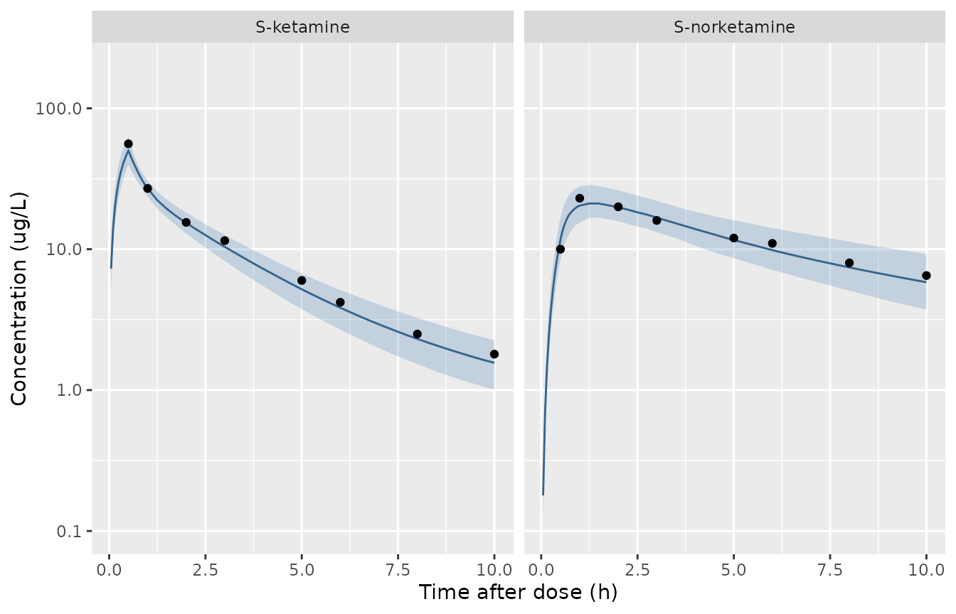
Replicates Figures 3b (S-ketamine) and 4b (S-norketamine) of Otto 2021: simulated median and 10th-90th percentiles (n = 200, CHDR1311 design) with the digitised observed median (points).
The typical-value (68 kg) solve is compared with the digitised observed medians at the sampling times. A transcription error in a clearance or volume, or a mass/unit slip in the metabolite flux, shifts a whole profile by tens of percent; the centre of the comparison is checked tightly and the envelope loosely, because each digitised point carries reading error.
chk_1311 <- typ_1311 |>
  filter(time %in% obs_median$time) |>
  select(time, `S-ketamine` = Cc_ugL, `S-norketamine` = Cc_snk_ugL) |>
  pivot_longer(-time, names_to = "analyte", values_to = "sim") |>
  inner_join(obs_median, by = c("time", "analyte")) |>
  mutate(pct_diff = 100 * (sim - conc) / conc)

chk_1311 |>
  mutate(sim = signif(sim, 3), pct_diff = round(pct_diff, 1)) |>
  rename(
    "Time (h)" = time, "Analyte" = analyte,
    "Typical-value simulation (ug/L)" = sim,
    "Observed median, digitised (ug/L)" = conc,
    "Difference (%)" = pct_diff
  ) |>
knitr::kable(caption = "Typical-value (68 kg) CHDR1311 prediction versus the digitised observed median.")| Time (h) | Analyte | Typical-value simulation (ug/L) | Observed median, digitised (ug/L) | Difference (%) |
|---|---|---|---|---|
| 0.5 | S-ketamine | 50.90 | 56.0 | -9.0 |
| 0.5 | S-norketamine | 11.80 | 10.0 | 18.1 |
| 1.0 | S-ketamine | 27.30 | 27.0 | 1.3 |
| 1.0 | S-norketamine | 20.90 | 23.0 | -9.3 |
| 2.0 | S-ketamine | 15.40 | 15.5 | -0.8 |
| 2.0 | S-norketamine | 20.50 | 20.0 | 2.4 |
| 3.0 | S-ketamine | 10.30 | 11.5 | -10.6 |
| 3.0 | S-norketamine | 17.10 | 16.0 | 6.8 |
| 5.0 | S-ketamine | 5.06 | 6.0 | -15.6 |
| 5.0 | S-norketamine | 11.70 | 12.0 | -2.4 |
| 6.0 | S-ketamine | 3.72 | 4.2 | -11.3 |
| 6.0 | S-norketamine | 9.90 | 11.0 | -10.0 |
| 8.0 | S-ketamine | 2.23 | 2.5 | -10.8 |
| 8.0 | S-norketamine | 7.41 | 8.0 | -7.3 |
| 10.0 | S-ketamine | 1.51 | 1.8 | -16.1 |
| 10.0 | S-norketamine | 5.79 | 6.5 | -11.0 |
chk_summary <- chk_1311 |>
  group_by(analyte) |>
  summarise(
    median_pct = median(pct_diff),
    q90_abs_pct = quantile(abs(pct_diff), 0.9),
    .groups = "drop"
  )
chk_summary
#> # A tibble: 2 × 3
#>   analyte       median_pct q90_abs_pct
#>   <chr>              <dbl>       <dbl>
#> 1 S-ketamine        -10.7         15.7
#> 2 S-norketamine      -4.90        13.1

stopifnot(
  all(abs(chk_summary$median_pct) < 15),
  all(chk_summary$q90_abs_pct < 25)
)
The S-ketamine typical profile sits about 10 percent below the observed median. That is the direction Otto 2021 reports for the same fixed S-ketamine parameters in Figure 3b: mean prediction error -1.27 ug/L (95 percent CI -1.99 to -0.50), a slight under-prediction.
The redeveloped model reproduces the S-norketamine peak at about 1 h and its level (about 21 ug/L predicted against about 23 ug/L observed), which was the stated purpose of the redevelopment: the Fanta 2015 metabolite sub-model under-predicted this Cmax (Otto 2021 Figure 4b).
CHDR1016: stepped 2-h infusion (Otto 2021 Figure 5 and Figure S1)
Figure 5 is a prediction-corrected VPC pooling both studies, which cannot be reproduced exactly without the observed data. The simulation below uses the Table 1 post-amendment high-occasion CHDR1016 regimen (0.026 mg/kg bolus, then 0.425, 0.275 and 0.15 mg/kg/h over 0-14, 15-39 and 40-120 min, with female rates increased by 5, 10 and 15 percent). Plotted against time after the end of infusion it shows the Figure 5 shape: an S-ketamine plateau near 100 ug/L before the stop, and an S-norketamine maximum near the stop that declines more slowly.
cohort_1016 <- data.frame(
  id = seq_len(n_sub),
  WT = draw_weight(n_sub, 71.3, 8.5),
  female = rbinom(n_sub, 1, 14 / 31)
)

make_events_1016 <- function(cohort) {
  seg <- data.frame(
    start = c(0, 14, 39) / 60,
    end = c(14, 39, 120) / 60,
    rate_kg = c(0.425, 0.275, 0.15),
    female_mult = c(1.05, 1.10, 1.15)
  )
  bolus <- cohort |>
    mutate(time = 0, amt = 0.026 * WT, rate = 0, evid = 1L, cmt = "central", dvid = NA_integer_)
  infusions <- tidyr::crossing(cohort, seg) |>
    mutate(
      rate = rate_kg * WT * ifelse(female == 1, female_mult, 1),
      amt = rate * (end - start),
      time = start, evid = 1L, cmt = "central", dvid = NA_integer_
    )
  obs <- tidyr::crossing(cohort, time = c(seq(0.05, 2, by = 0.05), seq(2.25, 7.5, by = 0.25))) |>
    mutate(amt = 0, rate = 0, evid = 0L, cmt = NA_character_, dvid = 1L)
  bind_rows(bolus, infusions, obs) |>
    arrange(id, time, desc(evid)) |>
    select(id, time, amt, rate, evid, cmt, dvid, WT)
}

sim_1016 <- rxode2::rxSolve(mod, make_events_1016(cohort_1016), keep = "WT") |>
  as.data.frame() |>
  mutate(Cc_ugL = Cc * 1000, Cc_snk_ugL = Cc_snk * 1000, tsi = time - 2)
sim_1016 |>
  select(id, tsi, `S-ketamine` = Cc_ugL, `S-norketamine` = Cc_snk_ugL) |>
  pivot_longer(-c(id, tsi), names_to = "analyte", values_to = "conc") |>
  group_by(tsi, analyte) |>
  summarise(
    med = median(conc), lo = quantile(conc, 0.1), hi = quantile(conc, 0.9),
    .groups = "drop"
  ) |>
  ggplot(aes(tsi, med)) +
  geom_ribbon(aes(ymin = lo, ymax = hi), alpha = 0.25, fill = "steelblue") +
  geom_line(colour = "steelblue4") +
  geom_vline(xintercept = 0, linetype = "dashed") +
  facet_wrap(~analyte) +
  scale_y_log10(limits = c(0.3, 500)) +
  labs(x = "Time after stop infusion (h)", y = "Concentration (ug/L)")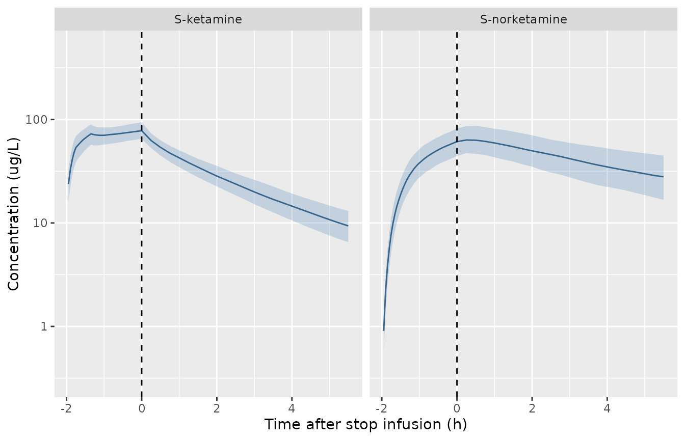
CHDR1016 high-occasion post-amendment regimen (n = 200): simulated median and 10th-90th percentiles against time after stop of infusion, the time axis of Otto 2021 Figure 5.
Individual parameter distributions (Otto 2021 Figure 2)
Figure 2 plots P_i = TVP * exp(eta) for the clearances
and central volumes of both analytes. The same draws from the packaged
OMEGA blocks (1000 parameter draws at 70 kg; no ODE solve) are shown
here.
ini_df <- mod$iniDf
om_k <- mod$omega[c("etalvc", "etalcl"), c("etalvc", "etalcl")]
om_n <- mod$omega[c("etalvc_snk", "etalcl_snk"), c("etalvc_snk", "etalcl_snk")]
set.seed(2021)
eta_k <- matrix(rnorm(2000), ncol = 2) %*% chol(om_k)
eta_n <- matrix(rnorm(2000), ncol = 2) %*% chol(om_n)
theta <- setNames(exp(ini_df$est), ini_df$name)

par_draws <- bind_rows(
  data.frame(analyte = "S-ketamine", parameter = "Central V (L)", value = theta[["lvc"]] * exp(eta_k[, 1])),
  data.frame(analyte = "S-ketamine", parameter = "CL (L/h)", value = theta[["lcl"]] * exp(eta_k[, 2])),
  data.frame(analyte = "S-norketamine", parameter = "Central V (L)", value = theta[["lvc_snk"]] * exp(eta_n[, 1])),
  data.frame(analyte = "S-norketamine", parameter = "CL (L/h)", value = theta[["lcl_snk"]] * exp(eta_n[, 2]))
)

ggplot(par_draws, aes(value, fill = analyte)) +
  geom_density(alpha = 0.4) +
  facet_wrap(~parameter, scales = "free") +
  labs(x = "Individual parameter value", y = "Density", fill = NULL)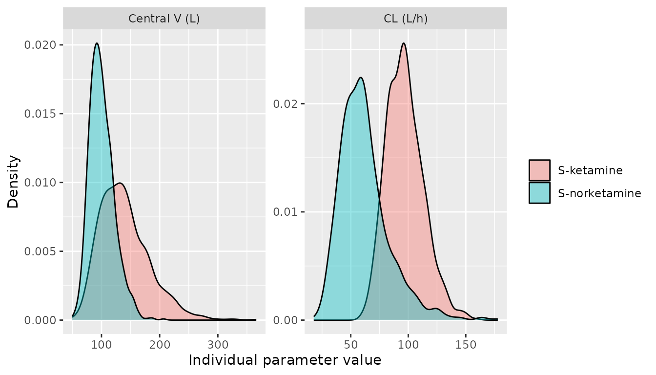
Replicates the final-model distributions in Otto 2021 Figure 2 (individual CL and central V of S-ketamine and S-norketamine at 70 kg).
PKNCA validation
Mass balance on the typical subject
With the fraction metabolised fixed at 1, every milligram of
S-ketamine cleared enters the S-norketamine compartment, so for a single
dose CL * AUCinf(S-ketamine) = Dose and
CL_snk * AUCinf(S-norketamine) = Dose. The check below runs
PKNCA on a deterministic typical-value (70 kg) solve of the 10 mg / 30
min CHDR1311 dose, sampled densely to 120 h so that the AUC
extrapolation is negligible. Both sides use the same drawn (typical)
parameters, so the difference is numerical only and a tight bound is
appropriate.
typ_times <- sort(unique(c(seq(0, 2, by = 0.02), seq(2.1, 24, by = 0.1), seq(24.5, 120, by = 0.5))))
ev_typ <- bind_rows(
  data.frame(id = 1L, time = 0, amt = 10, rate = 20, evid = 1L, cmt = "central", dvid = NA_integer_),
  data.frame(id = 1L, time = typ_times, amt = 0, rate = 0, evid = 0L, cmt = NA_character_, dvid = 1L)
) |>
  mutate(WT = 70)
typ70 <- rxode2::rxSolve(rxode2::zeroRe(mod), ev_typ) |> as.data.frame()
#> ℹ omega/sigma items treated as zero: 'etalvc', 'etalcl', 'etalvc_snk', 'etalcl_snk'

nca_long <- typ70 |>
  select(time, `S-ketamine` = Cc, `S-norketamine` = Cc_snk) |>
  pivot_longer(-time, names_to = "treatment", values_to = "Cc") |>
  mutate(id = 1L) |>
  filter(!is.na(Cc))

dose_typ <- data.frame(
  id = 1L, time = 0, amt = 10,
  treatment = c("S-ketamine", "S-norketamine")
)

nca_typ <- PKNCA::pk.nca(PKNCA::PKNCAdata(
  PKNCA::PKNCAconc(nca_long, Cc ~ time | treatment + id, concu = "mg/L", timeu = "h"),
  PKNCA::PKNCAdose(dose_typ, amt ~ time | treatment + id, doseu = "mg"),
  intervals = data.frame(start = 0, end = Inf, aucinf.obs = TRUE, cmax = TRUE, tmax = TRUE, half.life = TRUE)
))

res_typ <- as.data.frame(nca_typ) |>
  filter(PPTESTCD %in% c("aucinf.obs", "cmax", "tmax", "half.life")) |>
  select(treatment, PPTESTCD, PPORRES) |>
  pivot_wider(names_from = PPTESTCD, values_from = PPORRES)

cl_typ <- c("S-ketamine" = typ70$cl[1], "S-norketamine" = typ70$cl_snk[1])
res_typ <- res_typ |>
  mutate(
    cl = cl_typ[treatment],
    cl_times_auc = cl * aucinf.obs,
    pct_diff_vs_dose = 100 * (cl_times_auc - 10) / 10
  )

res_typ |>
  mutate(across(where(is.numeric), \(x) signif(x, 4))) |>
  rename(
    "Analyte" = treatment, "AUC0-inf (mg*h/L)" = aucinf.obs, "Cmax (mg/L)" = cmax,
    "Tmax (h)" = tmax, "t1/2 (h)" = half.life, "CL (L/h)" = cl,
    "CL x AUC0-inf (mg)" = cl_times_auc, "Difference from 10 mg dose (%)" = pct_diff_vs_dose
  ) |>
knitr::kable(caption = "PKNCA on the typical 70 kg subject after 10 mg S-ketamine over 30 min.")| Analyte | Cmax (mg/L) | Tmax (h) | t1/2 (h) | AUC0-inf (mg*h/L) | CL (L/h) | CL x AUC0-inf (mg) | Difference from 10 mg dose (%) |
|---|---|---|---|---|---|---|---|
| S-ketamine | 0.04987 | 0.50 | 7.328 | 0.1050 | 95.20 | 10 | -0.0001279 |
| S-norketamine | 0.02145 | 1.38 | 7.213 | 0.1732 | 57.72 | 10 | -0.0001030 |
Cohort NCA (CHDR1311 design)
conc_cohort <- sim_1311 |>
  select(id, time, `S-ketamine` = Cc, `S-norketamine` = Cc_snk) |>
  pivot_longer(-c(id, time), names_to = "treatment", values_to = "Cc") |>
  filter(!is.na(Cc))
dose_cohort <- tidyr::crossing(
  data.frame(id = cohort_1311$id, time = 0, amt = 10),
  treatment = c("S-ketamine", "S-norketamine")
)

nca_cohort <- PKNCA::pk.nca(PKNCA::PKNCAdata(
  PKNCA::PKNCAconc(conc_cohort, Cc ~ time | treatment + id, concu = "mg/L", timeu = "h"),
  PKNCA::PKNCAdose(dose_cohort, amt ~ time | treatment + id, doseu = "mg"),
  intervals = data.frame(start = 0, end = 10, cmax = TRUE, tmax = TRUE, auclast = TRUE)
))
knitr::kable(summary(nca_cohort), caption = "Simulated CHDR1311 NCA over 0-10 h (n = 200).")| Interval Start | Interval End | treatment | N | AUClast (h*mg/L) | Cmax (mg/L) | Tmax (h) |
|---|---|---|---|---|---|---|
| 0 | 10 | S-ketamine | 200 | 0.0937 [15.0] | 0.0501 [20.1] | 0.500 [0.500, 0.500] |
| 0 | 10 | S-norketamine | 200 | 0.120 [23.9] | 0.0215 [21.2] | 1.25 [0.950, 2.00] |
Comparison against published NCA
Otto 2021 reports no NCA table (no Cmax, Tmax, AUC or half-life values) for either study, so there is no published NCA to tabulate against. The quantitative comparison against the paper is the digitised CHDR1311 observed-median check above, together with the exact mass-balance identities.
Assumptions and deviations
-
S-norketamine is carried in S-ketamine mass units.
The supplementary NONMEM
$DESmoves S-ketamine amount into the S-norketamine compartment with no molecular-weight conversion (S-ketamine 237.7 g/mol, S-norketamine 223.7 g/mol), and the S-norketamine volume and clearance were estimated on measured S-norketamine mass concentrations. The packaged model keeps this as-run form; the estimated S-norketamine parameters absorb the 0.94 mass ratio, soCc_snkis directly comparable with measured S-norketamine concentrations in mass units. - Fraction metabolised fixed at 1. Otto 2021 states that, for identifiability, S-ketamine was assumed to be fully metabolised to S-norketamine. The S-norketamine volume and clearance are therefore apparent values.
- Peripheral parameters are not weight-scaled. Table 3 and the supplementary code scale only the central volumes and elimination clearances allometrically; Q1, Q2, Vp1 and Vp2 (and the S-norketamine Vp and Q) are weight-independent in the as-run model.
-
Estimated versus fixed. The six S-ketamine
population parameters are
fixed()(taken from Fanta 2015 and not re-estimated). The OMEGA, SIGMA and S-norketamine population values are the Otto 2021 estimates (Table 3 gives RSEs for them); the supplementary simulation code marks them FIX only because it is a simulation-only stream. The unrounded supplement values are used; they round to the Table 3 values. - Venous concentrations. Both studies and Fanta 2015 used venous sampling. The paper discusses that arterial concentrations are higher until the end of infusion; the model predicts venous concentrations only.
- Digitised targets. The CHDR1311 observed medians used in the quantitative check were read by the maintainers from the raster Figures 3b and 4b and carry about +/- 10 percent reading error.
- Virtual cohort. Weights are normal with the Table 1 mean and SD per study (redrawn beyond 3 SD); CHDR1016 female proportion 14/31. Only the post-amendment high-occasion CHDR1016 regimen is simulated.
- No errata were found for Otto 2021 (literature check 2026-09-28).