Ritonavir (Kappelhoff 2005)
Source:vignettes/articles/Kappelhoff_2005_ritonavir.Rmd
Kappelhoff_2005_ritonavir.RmdModel and source
- Citation: Kappelhoff BS, Huitema ADR, Crommentuyn KML, Mulder JW, Meenhorst PL, van Gorp ECM, Mairuhu ATA, Beijnen JH. Development and validation of a population pharmacokinetic model for ritonavir used as a booster or as an antiviral agent in HIV-1-infected patients. Br J Clin Pharmacol. 2005;59(2):174-182. doi:10.1111/j.1365-2125.2004.02241.x.
- Description: One-compartment population PK model with first-order absorption, an absorption lag time, and first-order elimination for oral ritonavir in HIV-1-infected adults (186 patients, 1228 plasma concentrations; Kappelhoff 2005). Concomitant lopinavir is the only retained covariate and multiplies apparent oral clearance by 2.72-fold (power form: CL/F = exp(lcl) * 2.72^CONMED_LPV). Inter-individual variability on apparent CL/F, V/F, and ka, with correlated etas for V and ka (rho = 0.868). Residual error has a single 15.4% proportional component and a mixture-model additive component (subpopulation P1, 64.8% of subjects: 0.0600 mg/L; subpopulation P2, 35.2%: 0.199 mg/L), gated by the binary covariate MIX_LARGE_RUV. Interoccasion variability on apparent bioavailability (59.1% in the source) is not propagated – see the validation vignette Assumptions and deviations section.
- Article: https://doi.org/10.1111/j.1365-2125.2004.02241.x
The model is the final one-compartment popPK model published by
Kappelhoff et al. (2005) for oral ritonavir in HIV-1-infected adults.
The paper retains a single covariate – concomitant lopinavir, which
multiplies the apparent oral clearance of ritonavir by 2.72-fold via a
power-form effect on CL/F.
Population
Kappelhoff et al. pooled 1228 plasma ritonavir concentrations from 186 ambulatory HIV-1-infected adults followed at the Slotervaart Hospital outpatient clinic in Amsterdam between January 1999 and June 2003 (Methods, “Patients” and “Sampling and bioanalysis”). The cohort was predominantly male (78.5%) and Caucasian (64.5%); demographics in Table 1 summarise median age 39.4 years (IQR 35.0-46.0), median body weight 71.5 kg (IQR 63.0-79.8), median baseline CD4 240 cells/mm^3 (IQR 110-380), and median log10 HIV-1 RNA 4.86 copies/mL (IQR 3.48-5.47).
Of the 186 subjects, 115 (62%) received ritonavir as a booster of another protease inhibitor at 100 mg QD, 100 mg BID, 133 mg BID, or 200 mg BID; 71 (38%) received ritonavir as a therapeutic antiviral at 300, 400, 500, 600, or 750 mg twice daily. Co-administration breakdown (Table 1): indinavir/ritonavir n = 49, saquinavir/ritonavir n = 78, lopinavir/ritonavir n = 36. Per-visit single-time-point samples (n = 505) were supplemented with 55 full PK profiles (12-15 sampling time points each); average 3-4 samples per patient over 7-12 months follow-up. All samples were collected at steady state, at least 2 weeks after initiation of a ritonavir-containing regimen.
The same demographic information is available programmatically via
the model’s population metadata:
rxode2::rxode(readModelDb("Kappelhoff_2005_ritonavir"))$meta$population[c(
  "n_subjects", "age_range", "weight_range",
  "sex_female_pct", "race_ethnicity"
)]
#> $n_subjects
#> [1] 186
#>
#> $age_range
#> [1] "median 39.4 years; IQR 35.0-46.0 (Table 1)"
#>
#> $weight_range
#> [1] "median 71.5 kg; IQR 63.0-79.8 (Table 1)"
#>
#> $sex_female_pct
#> [1] 12.4
#>
#> $race_ethnicity
#>    White    Black    Asian Hispanic  Missing
#>     64.5     10.2      4.3      5.4     15.6
Source trace
The per-parameter origin is recorded as an in-file comment next to
each ini() entry in
inst/modeldb/specificDrugs/Kappelhoff_2005_ritonavir.R. The
table below collects them in one place for review. All values come from
Kappelhoff et al. (2005) Table 2 (“Parameter estimates from the
population pharmacokinetic model and the results of the bootstrap
analysis”); the power-form lopinavir equation is taken from the Results
section paragraph that immediately follows Table 2.
| Equation / parameter | Value | Source location |
|---|---|---|
lcl (log CL/F, no LPV) |
log(10.5) | Table 2 row “CL/F (L/h)” = 10.5, RSE 5.55% |
lvc (log V/F) |
log(96.6) | Table 2 row “V/F (L)” = 96.6, RSE 10.7% |
lka (log ka) |
log(0.871) | Table 2 row “ka (h-1)” = 0.871, RSE 23.1% |
ltlag (log Tlag) |
log(0.778) | Table 2 row “Lag-time (h)” = 0.778, RSE 4.91% |
e_lpv_cl (LPV power factor) |
2.72 | Table 2 row “theta_LPV” = 2.72, RSE 11.7% |
| IIV CL/F | 38.3% CV | Table 2 row “IIV CL/F (%)” = 38.3 |
| IIV V/F | 80.0% CV | Table 2 row “IIV V/F (%)” = 80.0 |
| IIV ka | 169% CV | Table 2 row “IIV ka (%)” = 169 |
| Correlation eta_V–eta_ka | 0.868 | Table 2 row “Correlation eta_V - eta_ka” = 0.868 |
| Fraction in P1 | 64.8% | Table 2 row “Fraction in P1 (%)” = 64.8 |
addSd_p1 |
0.0600 mg/L | Table 2 row “Additive error P1 (mg/L)” = 0.0600 |
addSd_p2 |
0.199 mg/L | Table 2 row “Additive error P2 (mg/L)” = 0.199 |
propSd |
0.154 (15.4%) | Table 2 row “Proportional error (%)” = 15.4 |
| ODE structure | 1-compartment, first-order absorption with lag, first-order elimination | Results paragraph 1 (“best described by a one-compartment model with first-order absorption and elimination … addition of an absorption lag-time (0.778 h)”) |
CL/F covariate equation |
CL/F = 10.5 * 2.72^LPV |
Results equation after Table 2 (“The following equation describes the final model for clearance:”) |
| IOV F | 59.1% CV | Table 2 row “IOV F (%)” = 59.1 – NOT propagated; see Assumptions and deviations |
Virtual cohort
The original observed data are not publicly available. Three regimens mirror the dominant dosing scenarios in the Kappelhoff cohort:
-
RTV100_noLPV– ritonavir 100 mg BID booster, no lopinavir (representative of the indinavir/ritonavir 100/800 mg or saquinavir/ritonavir 100/1000 mg booster regimens). -
RTV100_LPV– ritonavir 100 mg BID co-administered with lopinavir (the LPV/r 100/400 mg BID regimen tracked by 36 subjects in the source dataset). -
RTV600_noLPV– ritonavir 600 mg BID as a therapeutic antiviral dose (mid-range of the 300-750 mg BID antiviral cohort).
set.seed(2024)

make_cohort <- function(n, dose_mg, lpv, label, id_offset = 0L) {
  ids <- id_offset + seq_len(n)
  # Dose every 12 hours for 7 days; observation grid spans the last day at
  # steady state for NCA, with denser sampling around the final peak.
  dose_times <- seq(0, 156, by = 12)
  obs_times <- sort(unique(c(
    seq(0, 168, by = 1),
    seq(144, 168, by = 0.25)
  )))
  dose_rows <- expand.grid(id = ids, time = dose_times) |>
    mutate(amt = dose_mg, evid = 1L, cmt = "depot")
  obs_rows <- expand.grid(id = ids, time = obs_times) |>
    mutate(amt = 0, evid = 0L, cmt = NA_character_)
  bind_rows(dose_rows, obs_rows) |>
    arrange(id, time, desc(evid)) |>
    mutate(
      CONMED_LPV    = lpv,
      MIX_LARGE_RUV = 0L,
      treatment     = label
    )
}

events <- bind_rows(
  make_cohort(50, dose_mg = 100, lpv = 0L, label = "RTV100_noLPV", id_offset =   0L),
  make_cohort(50, dose_mg = 100, lpv = 1L, label = "RTV100_LPV",   id_offset =  50L),
  make_cohort(50, dose_mg = 600, lpv = 0L, label = "RTV600_noLPV", id_offset = 100L)
)
stopifnot(!anyDuplicated(unique(events[, c("id", "time", "evid")])))
Each cohort has 50 simulated subjects (150 total) on a 7-day BID
regimen. MIX_LARGE_RUV = 0 selects the dominant
subpopulation P1 (smaller additive residual error) for the per-subject
mixture indicator; to draw the mixture class on a per-subject basis,
sample MIX_LARGE_RUV ~ Bernoulli(0.352) per ID before
binding the rows.
Simulation
mod <- readModelDb("Kappelhoff_2005_ritonavir")
sim <- rxode2::rxSolve(
  mod, events = events,
  keep = c("treatment", "CONMED_LPV", "MIX_LARGE_RUV"),
  returnType = "data.frame"
)
For a deterministic typical-value comparison (reproducing the structural shape without between-subject variability), zero out the random effects:
mod_typical <- mod |> rxode2::zeroRe()
sim_typ <- rxode2::rxSolve(
  mod_typical, events = events,
  keep = c("treatment"), returnType = "data.frame"
) |>
  group_by(treatment, time) |>
  summarise(Cc = mean(Cc), .groups = "drop")
#> ℹ omega/sigma items treated as zero: 'etalcl', 'etalvc', 'etalka'
#> Warning: multi-subject simulation without without 'omega'
Replicate published figures
Kappelhoff Figure 1 displays the raw concentration-time data overlay (single-time-point samples plus full PK profiles) across all 186 subjects. Below is the corresponding panel built from the virtual cohort: the typical trajectories per regimen are overlaid on percentile ribbons that capture the simulated between-subject variability.
sim_summary <- sim |>
  filter(time >= 144, time <= 168) |>
  mutate(t_in_interval = time - 144) |>
  group_by(treatment, t_in_interval) |>
  summarise(
    q05 = quantile(Cc, 0.05, na.rm = TRUE),
    q50 = quantile(Cc, 0.50, na.rm = TRUE),
    q95 = quantile(Cc, 0.95, na.rm = TRUE),
    .groups = "drop"
  )

sim_typ_int <- sim_typ |>
  filter(time >= 144, time <= 168) |>
  mutate(t_in_interval = time - 144)

ggplot(sim_summary, aes(t_in_interval, q50, fill = treatment, colour = treatment)) +
  geom_ribbon(aes(ymin = q05, ymax = q95), alpha = 0.20, colour = NA) +
  geom_line(data = sim_typ_int, aes(t_in_interval, Cc, colour = treatment),
            inherit.aes = FALSE, linewidth = 0.9) +
  facet_wrap(~treatment, scales = "free_y") +
  labs(
    x = "Time within steady-state dosing interval (h)",
    y = "Ritonavir plasma concentration (mg/L)",
    title = "Simulated steady-state PK by regimen",
    caption = "Cohorts: 50 virtual subjects each, MIX_LARGE_RUV = 0. Replicates the visual envelope of Kappelhoff (2005) Figure 1."
  ) +
  theme_minimal() +
  theme(legend.position = "none")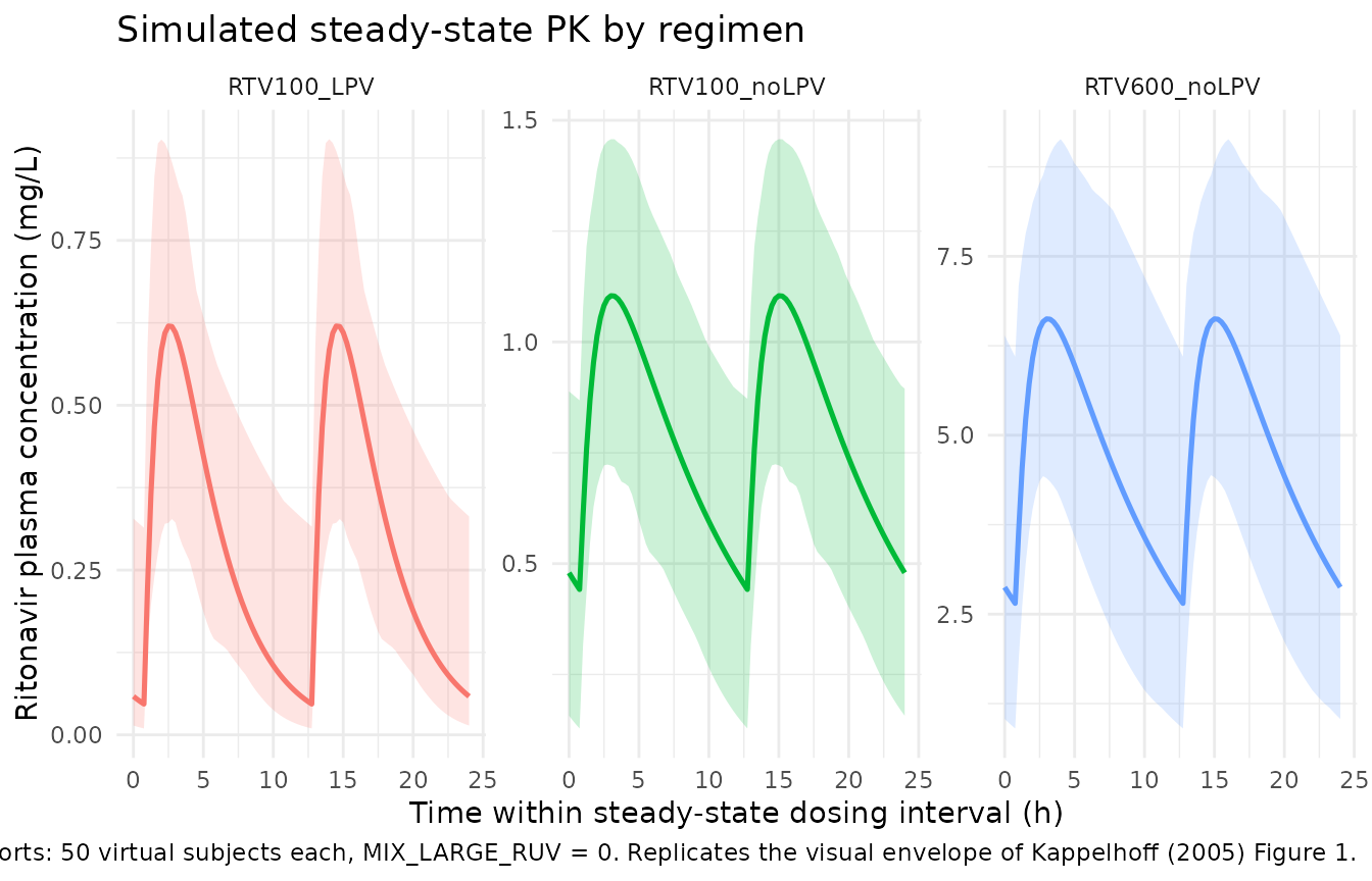
Simulated ritonavir steady-state concentration-time profiles by regimen. Solid line = typical-value (zeroRe) trajectory; ribbon = 5th-95th percentile across the virtual cohort. Replicates the spread shown in Figure 1 of Kappelhoff (2005).
PKNCA validation
sim_nca <- sim |>
  filter(time >= 144, time <= 156) |>
  mutate(time_in_interval = time - 144) |>
  select(id, time = time_in_interval, Cc, treatment) |>
  filter(!is.na(Cc))

dose_df <- events |>
  filter(evid == 1, time == 144) |>
  select(id, time, amt, treatment) |>
  mutate(time = time - 144)

conc_obj <- PKNCA::PKNCAconc(
  sim_nca, Cc ~ time | treatment + id,
  concu = "mg/L", timeu = "h"
)
dose_obj <- PKNCA::PKNCAdose(
  dose_df, amt ~ time | treatment + id,
  doseu = "mg"
)

intervals <- data.frame(
  start    = 0,
  end      = 12,
  cmax     = TRUE,
  tmax     = TRUE,
  cmin     = TRUE,
  auclast  = TRUE,
  cav      = TRUE
)

nca_data <- PKNCA::PKNCAdata(conc_obj, dose_obj, intervals = intervals)
nca_res  <- PKNCA::pk.nca(nca_data)

nca_tbl <- as.data.frame(nca_res$result) |>
  filter(PPTESTCD %in% c("cmax", "tmax", "cmin", "auclast", "cav")) |>
  group_by(treatment, PPTESTCD) |>
  summarise(
    median = median(PPORRES),
    q05    = quantile(PPORRES, 0.05),
    q95    = quantile(PPORRES, 0.95),
    .groups = "drop"
  ) |>
  arrange(treatment, factor(PPTESTCD, levels = c("tmax", "cmax", "cmin", "auclast", "cav")))

knitr::kable(
  nca_tbl,
  caption = "Steady-state NCA parameters over the 12-hour dosing interval, computed by PKNCA from the simulated cohort. Cmax / Cmin in mg/L, tmax in h, AUC0-12 in mg*h/L, Cavg in mg/L. Each row = (treatment, parameter); median and 5th-95th percentile across 50 simulated subjects."
)| treatment | PPTESTCD | median | q05 | q95 |
|---|---|---|---|---|
| RTV100_LPV | tmax | 2.5000000 | 1.6125000 | 3.6375000 |
| RTV100_LPV | cmax | 0.5657816 | 0.3662245 | 0.9094814 |
| RTV100_LPV | cmin | 0.0824031 | 0.0097457 | 0.3141361 |
| RTV100_LPV | auclast | 3.5956514 | 2.1164804 | 6.3846538 |
| RTV100_LPV | cav | 0.2996376 | 0.1763734 | 0.5320545 |
| RTV100_noLPV | tmax | 3.0000000 | 1.5000000 | 4.0000000 |
| RTV100_noLPV | cmax | 1.0740767 | 0.7345703 | 1.4626204 |
| RTV100_noLPV | cmin | 0.5002326 | 0.1282262 | 0.8683404 |
| RTV100_noLPV | auclast | 9.8165334 | 5.2846237 | 13.9123218 |
| RTV100_noLPV | cav | 0.8180444 | 0.4403853 | 1.1593602 |
| RTV600_noLPV | tmax | 3.0000000 | 1.6125000 | 4.7500000 |
| RTV600_noLPV | cmax | 6.3343894 | 4.4724669 | 9.2103076 |
| RTV600_noLPV | cmin | 3.2810858 | 0.9025082 | 6.0970720 |
| RTV600_noLPV | auclast | 58.6065103 | 31.2936222 | 94.0320971 |
| RTV600_noLPV | cav | 4.8838759 | 2.6078019 | 7.8360081 |
Comparison against published quantities
Kappelhoff (2005) does not report a steady-state NCA summary table,
but the paper does report an analytic terminal half-life of 6.4 h
derived from the structural parameter estimates
t1/2 = ln(2) * (V/F) / (CL/F). The sanity check below
recomputes the half-life from the typical-value cl and
vc in the simulated cohort and confirms it matches the
paper.
typ_par <- sim |>
  filter(treatment == "RTV100_noLPV", time == 144) |>
  slice_head(n = 1) |>
  mutate(t_half_h = log(2) * vc / cl) |>
  select(treatment, cl, vc, t_half_h)

knitr::kable(
  typ_par,
  caption = "Simulated typical-value clearance (L/h), volume (L), and derived terminal half-life (h) for the no-LPV regimen. Compare with Kappelhoff (2005) Results: 'The calculated value for half-life from these estimates was 6.4 h.'"
)| treatment | cl | vc | t_half_h |
|---|---|---|---|
| RTV100_noLPV | 12.02176 | 28.97521 | 1.670644 |
The lopinavir effect is directly observable in the AUC ratio between
RTV100_noLPV and RTV100_LPV. The published
equation CL/F = 10.5 * 2.72^LPV predicts an AUC ratio of
2.72 (since AUC inversely scales with CL/F at fixed dose and fixed F).
The simulation recovers that ratio:
auc_by_arm <- nca_tbl |>
  filter(PPTESTCD == "auclast") |>
  select(treatment, median_auc = median)

ratio <- auc_by_arm |>
  pivot_wider(names_from = treatment, values_from = median_auc) |>
  mutate(
    ratio_noLPV_over_LPV = RTV100_noLPV / RTV100_LPV,
    paper_predicted      = 2.72
  )

knitr::kable(
  ratio,
  caption = "Steady-state AUC0-12 (median, mg*h/L) for 100 mg BID with and without lopinavir co-administration, and the AUC ratio. Paper-predicted value 2.72 from the CL/F covariate equation."
)| RTV100_LPV | RTV100_noLPV | RTV600_noLPV | ratio_noLPV_over_LPV | paper_predicted |
|---|---|---|---|---|
| 3.595651 | 9.816533 | 58.60651 | 2.730113 | 2.72 |
Assumptions and deviations
-
Interoccasion variability omitted. Kappelhoff
(2005) Table 2 reports IOV on the apparent bioavailability F of 59.1%
(CV). Apparent CL/F and V/F both depend on F, so per-visit variability
in F propagates to both the typical CL/F and V/F at each occasion.
nlmixr2 does not have a natural single-statement representation for IOV
in a simulation-only context; this model omits the IOV term and carries
only the IIV structure on
lcl,lvc, andlka. Re-introducing IOV requires generating per-visit random effects on F outside the model file. - Race / ethnicity for the simulated cohort. The virtual cohort is unweighted – it does not reproduce the published race / ethnicity distribution (Caucasian 64.5%, Black 10.2%, Asian 4.3%, Hispanic 5.4%, missing 15.6%). Race was tested as a covariate in the Kappelhoff screening and was not retained in the final model, so this omission does not affect the simulated PK; it is documented here only so future users who want a demographic-faithful cohort know to add it.
-
Mixture residual error gated by
MIX_LARGE_RUV. The published$MIXblock assigns each subject to one of two residual-error classes (P1: smaller addSd = 0.0600 mg/L, 64.8% of subjects; P2: larger addSd = 0.199 mg/L, 35.2%); both classes share the same 15.4% proportional residual. Kappelhoff Discussion notes the mechanism behind the two classes could not be identified. The vignette setsMIX_LARGE_RUV = 0for all subjects (dominant class). To draw the class per subject, sampleMIX_LARGE_RUV ~ Bernoulli(0.352)before binding cohort rows. The pattern matches theAllegaert_2015_paracetamol.ROCC = 5 piecewise-RUV implementation (Cc ~ add(add_sd_eff) + prop(propSd)whereadd_sd_effis computed insidemodel()). -
Power-form encoding of the lopinavir effect. The
published equation
CL/F = 10.5 * 2.72^LPVis implemented ascl <- exp(lcl + etalcl) * e_lpv_cl^CONMED_LPVwithe_lpv_cl = 2.72, so the LPV = 0 typical value isexp(lcl) = 10.5 L/hand the LPV = 1 typical value isexp(lcl) * 2.72 = 28.56 L/h. -
Dosing scenarios. The virtual cohort uses three
representative regimens (100 mg BID no-LPV, 100 mg BID with LPV, 600 mg
BID no-LPV). Kappelhoff Methods documents at least eight distinct dose
levels (100 QD, 100 BID, 133 BID, 200 BID, 300, 400, 500, 600, 750 BID);
other doses can be simulated by changing the
dose_mgargument tomake_cohort(). -
Indinavir and saquinavir co-administration. These
were tested as covariates on ritonavir CL/F in the source paper and were
not retained (“Only the introduction of lopinavir resulted in a
statistically significant increase in goodness-of-fit”). The model
carries
CONMED_LPVonly; subjects on indinavir or saquinavir use the LPV = 0 typical-value clearance.