Model and source
- Citation: Zhang X, Peyret T, Gosselin NH, Marier JF, Imel EA, Carpenter TO. Population Pharmacokinetic and Pharmacodynamic Analyses From a 4-Month Intradose Escalation and Its Subsequent 12-Month Dose Titration Studies for a Human Monoclonal Anti-FGF23 Antibody (KRN23) in Adults With X-Linked Hypophosphatemia. J Clin Pharmacol. 2016;56(4):429-438. doi:10.1002/jcph.611
- Description: One-compartment population PK model with first-order absorption for subcutaneous burosumab (development code KRN23, a human anti-FGF23 IgG1 monoclonal antibody) in adults with X-linked hypophosphatemia, coupled to an Emax pharmacodynamic model for the change from baseline in serum phosphate (Pi) in which the potency EC50 drifts upward over treatment time. Apparent clearance and apparent central volume carry fixed allometric exponents on body weight (0.75 and 1) referenced to 70 kg, and CL/F is 1.15-fold higher at the lowest studied dose level (0.05 mg/kg) than over the linear 0.1 to 1.0 mg/kg range. The PD potency EC50,t rises sigmoidally with time since the first dose, from 1799.6 ng/mL at time 0 toward an asymptote 4605.5 ng/mL higher, with a half-maximal rise at a structurally fixed 32 weeks; this captures the loss of phosphate response observed after roughly 280 days of monthly dosing.
- Article: https://doi.org/10.1002/jcph.611
Burosumab is the INN for the anti-FGF23 monoclonal antibody that Zhang 2016 calls by its development code, KRN23. This vignette uses the INN throughout; the paper’s own tables and equations are cited with the paper’s notation.
Population
The model was built from three studies in adults with X-linked hypophosphatemia (XLH): the single-dose study KRN23-US-02 (NCT00830674), the 4-month intradose-escalation study KRN23-INT-001 (NCT01340482), and its 12-month titration extension KRN23-INT-002 (NCT01571596).
The PK analysis set is 40 subjects contributing 1192 measurable serum burosumab concentrations: 12 subcutaneously dosed subjects from KRN23-US-02 (200 concentrations, sampled to day 50) plus the 28 subjects of KRN23-INT-001 (719 concentrations), with 273 further concentrations from KRN23-INT-002. Intravenous single-dose data were excluded because subcutaneous bioavailability was essentially complete. The PD analysis set is the 28 multiple-dose subjects, contributing 1621 serum phosphate (Pi) observations; 22 of them continued into the extension and 19 received all 16 doses.
Baseline characteristics are in Zhang 2016 Table 1. Subjects were 25 to 68 years old in KRN23-US-02 (48 +/- 11 years) and had a lower age bound of 20 years in the two multiple-dose studies (42 +/- 14 and 42 +/- 15 years); body weight spanned 46 to 124 kg across the three studies, and the cohort was predominantly female (25 of the 40 PK-analysis subjects) and almost entirely white (a single African American participant per multiple-dose study). The disease signature is visible at baseline: serum Pi (1.6 to 1.9 mg/dL) and TmP/GFR (1.6 to 1.9 mg/dL) both sat below their normal ranges, while median intact FGF23 was above the upper limit of normal.
The same information is available programmatically via the model’s
population metadata
(readModelDb("Zhang_2016_burosumab")()$population).
Source trace
The per-parameter origin is recorded as an in-file comment next to
each ini() entry in
inst/modeldb/specificDrugs/Zhang_2016_burosumab.R. The
table below collects them in one place for review.
| Equation / parameter | Value | Source location |
|---|---|---|
lka |
0.349 /day | Table 2, Ka (90%CI 0.300-0.398, RSE 7.2%) |
lcl |
0.279 L/day | Table 2, CL/F at 70 kg for doses >= 0.1 mg/kg (90%CI
0.247-0.311, RSE 5.1%) |
lvc |
7.17 L | Table 2, Vc/F at 70 kg (90%CI 6.45-7.89, RSE 5.1%) |
e_wt_cl |
0.75 (fixed) | Table 2, (WT/70)^0.75 on CL/F; Methods, allometry “as
proposed for monoclonal antibodies” |
e_wt_vc |
1 (fixed) | Table 2, (WT/70)^1 on Vc/F |
e_dose_low_cl |
1.15 | Table 2, CL/F at 0.05 mg/kg = 0.321 = 1.15 x typical (90%CI 1.109-1.194, RSE 1.9%) |
etalka |
0.155378 | Table 2, BSV Ka 41.0%; log(0.410^2 + 1)
|
etalcl |
0.127006 | Table 2, BSV CL/F 36.8%; log(0.368^2 + 1)
|
etalvc |
0.088949 | Table 2, BSV Vc/F 30.5%; log(0.305^2 + 1)
|
propSd |
0.218 | Table 2, Error prop 21.8% (90%CI 7.7%-35.8%) |
addSd |
0.099 ng/mL | Table 2, Error additive (90%CI 0.054-0.144) |
lemax |
1.5 mg/dL (fixed) | Table 3, Emax (FIX); note to Table 3 |
ltvec50 |
1799.6 ng/mL | Table 3, tvEC50 (RSE 15.9%) |
lec50_time_max |
4605.5 ng/mL | Table 3, a (RSE 16.8%) |
lec50_time_hill |
2.88 | Table 3, g (RSE 17.1%) |
lec50_t50 |
32 weeks (fixed) | Equation 10 denominator, (32^g + t^g); not in Table
3 |
etaltvec50 |
0.434793 | Table 3, BSV EC50,t 73.8%; log(0.738^2 + 1)
|
addSd_dPi |
0.310 mg/dL | Table 3, Residual additive error (RSE 1.8%) |
| Structural model: 1 compartment, first-order absorption, no lag | n/a | Results “KRN23 Population Pharmacokinetics”; Supplementary Table S1 |
| Dose-level effect on CL/F | n/a | Results; Supplementary Table S2 (dMOF 37.117) |
dPi = Emax * C / (EC50,t + C) |
n/a | Equation 9, page 435 |
EC50,t = tvEC50 + a * t^g / (32^g + t^g), t in
weeks |
n/a | Equation 10, page 435 |
Two features of equation 10 that Table 3 does not record
Both are flagged here because a reader working from Table 3 alone would not recover the published EC50,t values.
-
The 32 in the denominator is a structural constant.
It appears only inside the printed equation and has no row in Table 3.
The model file carries it as the fixed parameter
ec50_t50(32 weeks) so it is visible and source-traced rather than buried as a magic number. -
ais an increment, not a rate. Table 3 gives its units as ng/mL/week and its footnote calls it the “maximum rate of increase of EC50,t”, but in equation 10 it multiplies a dimensionless saturating function of time, so dimensionally and functionally it is the asymptotic increase of EC50,t in ng/mL. The gate below confirms this reading reproduces all three EC50,t values quoted in the paper; the “rate” reading cannot.
Model structure
mod <- readModelDb("Zhang_2016_burosumab")
ui <- rxode2::rxode(mod)
ui
#>  ── rxode2-based free-form 2-cmt ODE model ──────────────────────────────────────
#>  ── Initalization: ──
#> Fixed Effects ($theta):
#>             lka             lcl             lvc         e_wt_cl         e_wt_vc
#>      -1.0526834      -1.2765435       1.9699057       0.7500000       1.0000000
#>   e_dose_low_cl          propSd           addSd           lemax         ltvec50
#>       1.1500000       0.2180000       0.0990000       0.4054651       7.4953197
#>  lec50_time_max lec50_time_hill       lec50_t50       addSd_dPi
#>       8.4350065       1.0577903       3.4657359       0.3100000
#>
#> Omega ($omega):
#>              etalka   etalcl   etalvc etaltvec50
#> etalka     0.155378 0.000000 0.000000   0.000000
#> etalcl     0.000000 0.127006 0.000000   0.000000
#> etalvc     0.000000 0.000000 0.088949   0.000000
#> etaltvec50 0.000000 0.000000 0.000000   0.434793
#>
#> States ($state or $stateDf):
#>   Compartment Number Compartment Name
#> 1                  1            depot
#> 2                  2          central
#>  ── Multiple Endpoint Model ($multipleEndpoint): ──
#>   variable                cmt                dvid*
#> 1   Cc ~ …  cmt='Cc' or cmt=3  dvid='Cc' or dvid=1
#> 2  dPi ~ … cmt='dPi' or cmt=4 dvid='dPi' or dvid=2
#>   * If dvids are outside this range, all dvids are re-numered sequentially, ie 1,7, 10 becomes 1,2,3 etc
#>
#>  ── μ-referencing ($muRefTable): ──
#>   theta    eta level
#> 1   lka etalka    id
#> 2   lcl etalcl    id
#> 3   lvc etalvc    id
#>
#>  ── Model (Normalized Syntax): ──
#> function() {
#>     compartmentData <- list(depot = list(analyte = "burosumab",
#>         units = "mg", specimen = "administration site", verified = TRUE),
#>         central = list(analyte = "burosumab", units = "mg", specimen = "serum",
#>             verified = TRUE))
#>     covariateData <- list(WT = list(description = "Body weight at baseline",
#>         units = "kg", type = "continuous", reference_category = NULL,
#>         notes = "Allometric scaling referenced to 70 kg, with exponents fixed at 0.75 on CL/F and 1 on Vc/F (Zhang 2016 Table 2). Body weight was the only covariate retained in the final PK model; Zhang 2016 Discussion notes that model-predicted steady-state AUC at 0.1 mg/kg is independent of body weight (Supplementary Figure S3), i.e. the mg/kg dosing plus the allometric terms together flatten the exposure-weight relationship.",
#>         source_name = "WT"), DOSE_LOW = list(description = "Lowest studied burosumab dose level indicator",
#>         units = "(binary)", type = "binary", reference_category = "0 (0.1, 0.3, 0.6 or 1.0 mg/kg subcutaneous burosumab)",
#>         notes = "1 = the dose record is the 0.05 mg/kg dose level, which in study KRN23-INT-001 is the first step of the four-step intradose escalation (0.05 -> 0.1 -> 0.3 -> 0.6 mg/kg); 0 = any of the 0.1, 0.3, 0.6 or 1.0 mg/kg levels. Time-varying within a subject, not subject-level: a KRN23-INT-001 participant carries DOSE_LOW = 1 only during the first 28-day dosing interval and 0 thereafter. Zhang 2016 Results 'KRN23 Population Pharmacokinetics' fit a separate typical CL/F per dose level (0.320 L/day at 0.05 mg/kg vs 0.271-0.294 L/day from 0.1 to 1.0 mg/kg, Supplementary Table S2), concluded the PK was linear from 0.1 to 1.0 mg/kg, and therefore pooled the higher levels against a single low-dose multiplier (dMOF 37.117). Zhang 2016 Discussion attributes the higher low-dose CL/F to free circulating intact FGF23 acting as a target sink that is proportionally more important at low burosumab concentrations.",
#>         source_name = "dose level"))
#>     covariatesDataExcluded <- list(AGE = list(description = "Age",
#>         units = "years", type = "continuous", notes = "Screened graphically against BSV on CL/F and Vc/F; not retained (Zhang 2016 Methods 'Population PK Methodology' and Results)."),
#>         SEXF = list(description = "Female sex indicator", units = "(binary)",
#>             type = "binary", notes = "Screened via box plots; not retained (Zhang 2016 Methods 'Population PK Methodology' and Results)."),
#>         RACE_BLACK = list(description = "African American race indicator",
#>             units = "(binary)", type = "binary", notes = "Screened; not retained. The cohort was 60/62 white with a single African American participant per multiple-dose study (Zhang 2016 Table 1), so race was not estimable."),
#>         FGF23 = list(description = "Baseline intact fibroblast growth factor 23",
#>             units = "pg/mL", type = "continuous", notes = "Screened as an intrinsic factor on CL/F and Vc/F; not retained as a covariate, although Zhang 2016 Discussion invokes free intact FGF23 to explain the higher CL/F at 0.05 mg/kg that is instead encoded by DOSE_LOW."),
#>         BALP = list(description = "Baseline bone alkaline phosphatase",
#>             units = "ug/L", type = "continuous", notes = "Screened as an intrinsic factor; not retained (Zhang 2016 Methods 'Population PK Methodology')."))
#>     description <- "One-compartment population PK model with first-order absorption for subcutaneous burosumab (development code KRN23, a human anti-FGF23 IgG1 monoclonal antibody) in adults with X-linked hypophosphatemia, coupled to an Emax pharmacodynamic model for the change from baseline in serum phosphate (Pi) in which the potency EC50 drifts upward over treatment time. Apparent clearance and apparent central volume carry fixed allometric exponents on body weight (0.75 and 1) referenced to 70 kg, and CL/F is 1.15-fold higher at the lowest studied dose level (0.05 mg/kg) than over the linear 0.1 to 1.0 mg/kg range. The PD potency EC50,t rises sigmoidally with time since the first dose, from 1799.6 ng/mL at time 0 toward an asymptote 4605.5 ng/mL higher, with a half-maximal rise at a structurally fixed 32 weeks; this captures the loss of phosphate response observed after roughly 280 days of monthly dosing."
#>     population <- list(species = "human", n_subjects = 40, n_studies = 3,
#>         age_range = "25-68 years (KRN23-US-02); lower bound 20 years in KRN23-INT-001 / KRN23-INT-002 (the printed upper bound is not legible in the source PDF)",
#>         age_median = "48 +/- 11 years (KRN23-US-02, mean +/- SD); 42 +/- 14 (KRN23-INT-001); 42 +/- 15 (KRN23-INT-002)",
#>         weight_range = "48-103 kg (KRN23-US-02); 46-122 kg (KRN23-INT-001); 51-124 kg (KRN23-INT-002)",
#>         weight_median = "73 +/- 16 kg (KRN23-US-02, mean +/- SD); 70 kg median (KRN23-INT-001); 75.3 kg median (KRN23-INT-002)",
#>         sex_female_pct = 62.5, race_ethnicity = c(White = 97.5,
#>             Black = 2.5), disease_state = "X-linked hypophosphatemia (XLH) in adults; baseline serum Pi 1.6-1.9 mg/dL and TmP/GFR 1.6-1.9 mg/dL, both below the normal ranges, with median intact FGF23 above the upper limit of normal",
#>         dose_range = "0.05-1.0 mg/kg subcutaneous every 28 days; 0.1-1.0 mg/kg subcutaneous single dose",
#>         regions = "United States and international sites (NCT00830674, NCT01340482, NCT01571596)",
#>         notes = "Baseline demographics and laboratory values are in Zhang 2016 Table 1. PK analysis set: 40 subjects (12 from the single-dose study KRN23-US-02 plus 28 from the dose-escalation study KRN23-INT-001) contributing 1192 measurable KRN23 concentrations. PD analysis set: the 28 multiple-dose subjects contributing 1621 serum Pi observations; 22 of them continued into the 12-month extension KRN23-INT-002 and 19 received all 16 doses. IV single-dose data were excluded because subcutaneous bioavailability was essentially complete. Sex percentages are pooled across the three study columns of Table 1 (24 female of 62 study entries is 38.7% male / 61.3% female; the value here uses the 40-subject PK analysis set: 6 + 19 = 25 female of 40).")
#>     reference <- "Zhang X, Peyret T, Gosselin NH, Marier JF, Imel EA, Carpenter TO. Population Pharmacokinetic and Pharmacodynamic Analyses From a 4-Month Intradose Escalation and Its Subsequent 12-Month Dose Titration Studies for a Human Monoclonal Anti-FGF23 Antibody (KRN23) in Adults With X-Linked Hypophosphatemia. J Clin Pharmacol. 2016;56(4):429-438. doi:10.1002/jcph.611"
#>     units <- list(time = "day", dosing = "mg", concentration = "ng/mL")
#>     vignette <- "Zhang_2016_burosumab"
#>     ini({
#>         lka <- -1.05268335677971
#>         label("First-order absorption rate constant (1/day)")
#>         lcl <- -1.27654349716077
#>         label("Apparent clearance CL/F at 70 kg, doses >= 0.1 mg/kg (L/day)")
#>         lvc <- 1.96990565461153
#>         label("Apparent central volume Vc/F at 70 kg (L)")
#>         e_wt_cl <- fix(0.75)
#>         label("Allometric exponent of body weight on CL/F (unitless)")
#>         e_wt_vc <- fix(1)
#>         label("Allometric exponent of body weight on Vc/F (unitless)")
#>         e_dose_low_cl <- 1.15
#>         label("Fold-increase in CL/F at the 0.05 mg/kg dose level (unitless)")
#>         propSd <- c(0, 0.218)
#>         label("Proportional residual error on serum burosumab (fraction)")
#>         addSd <- c(0, 0.099)
#>         label("Additive residual error on serum burosumab (ng/mL)")
#>         lemax <- fix(0.405465108108164)
#>         label("Maximum effect on serum Pi change from baseline (mg/dL)")
#>         ltvec50 <- 7.49531969696702
#>         label("EC50,t at time zero, tvEC50 (ng/mL)")
#>         lec50_time_max <- 8.43500652042829
#>         label("Maximum increase of EC50,t above tvEC50 (ng/mL)")
#>         lec50_time_hill <- 1.05779029414785
#>         label("Hill coefficient of the EC50,t rise over time (unitless)")
#>         lec50_t50 <- fix(3.46573590279973)
#>         label("Time to half-maximal rise of EC50,t (weeks)")
#>         addSd_dPi <- c(0, 0.31)
#>         label("Additive residual error on serum Pi change from baseline (mg/dL)")
#>         etalka ~ 0.155378
#>         etalcl ~ 0.127006
#>         etalvc ~ 0.088949
#>         etaltvec50 ~ 0.434793
#>     })
#>     model({
#>         ka <- exp(lka + etalka)
#>         cl <- exp(lcl + etalcl) * (WT/70)^e_wt_cl * e_dose_low_cl^DOSE_LOW
#>         vc <- exp(lvc + etalvc) * (WT/70)^e_wt_vc
#>         kel <- cl/vc
#>         d/dt(depot) <- -ka * depot
#>         d/dt(central) <- ka * depot - kel * central
#>         Cc <- 1000 * central/vc
#>         tweek <- t/7
#>         tvec50 <- exp(ltvec50 + etaltvec50)
#>         ec50_time_max <- exp(lec50_time_max + etaltvec50)
#>         ec50_time_hill <- exp(lec50_time_hill)
#>         ec50_t50 <- exp(lec50_t50)
#>         ec50t <- tvec50 + ec50_time_max * tweek^ec50_time_hill/(ec50_t50^ec50_time_hill +
#>             tweek^ec50_time_hill)
#>         emax <- exp(lemax)
#>         dPi <- emax * Cc/(ec50t + Cc)
#>         Cc ~ add(addSd) + prop(propSd)
#>         dPi ~ add(addSd_dPi)
#>     })
#> }
Structural gates
Gate 1: the solved PK matches its own closed form
The disposition is one compartment with first-order input, so the typical-value solution has an exact closed form. Both sides use the same parameters, so the only difference is integration error and the bound is correspondingly tight.
mod_typ <- mod |> rxode2::zeroRe()

single_dose_events <- function(dose_mg, wt = 70, dose_low = 0L,
                               times = seq(0, 140, by = 0.5), id = 1L) {
  n <- length(times)
  data.frame(
    id       = id,
    time     = c(0, times),
    amt      = c(dose_mg, rep(NA_real_, n)),
    evid     = c(1L, rep(0L, n)),
    cmt      = c("depot", rep("central", n)),
    # dvid = 1 tags every observation row with the first endpoint (Cc). The
    # model declares two endpoints (Cc and dPi), so rxode2 needs the endpoint
    # mapping; every algebraic observable is still returned as a column.
    dvid     = c(NA_integer_, rep(1L, n)),
    WT       = wt,
    DOSE_LOW = dose_low
  )
}

ev1 <- single_dose_events(dose_mg = 70)
sim1 <- rxode2::rxSolve(mod_typ, events = ev1, useLinCmt = FALSE,
                        returnType = "data.frame")
#> ℹ omega/sigma items treated as zero: 'etalka', 'etalcl', 'etalvc', 'etaltvec50'

ka <- 0.349
cl <- 0.279
vc <- 7.17
kel <- cl / vc
closed_form <- 1000 * (70 * ka / (vc * (ka - kel))) *
  (exp(-kel * sim1$time) - exp(-ka * sim1$time))

rel_err <- max(abs(sim1$Cc - closed_form) / pmax(closed_form, 1e-9))
rel_err
#> [1] 3.850658e-07

stopifnot(rel_err < 1e-5)
Gate 2: derived constants match the values quoted in the text
Zhang 2016 Discussion states an elimination rate constant of 0.03891 /day (= 0.279 / 7.17), an elimination half-life of about 17.8 days, and an absorption half-life of approximately 2.0 days.
derived <- tibble::tibble(
  Quantity = c("kel (1/day)", "Elimination half-life (day)",
               "Absorption half-life (day)", "Tmax after a single dose (day)"),
  Model = c(kel, log(2) / kel, log(2) / ka, log(ka / kel) / (ka - kel)),
  Published = c(0.03891, 17.8, 2.0, NA_real_),
  Source = c("Discussion, p. 437", "Discussion, p. 437", "Discussion, p. 436",
             "cf. Abstract: peak serum Pi 7-10 days after dosing")
)
knitr::kable(derived, digits = c(0, 5, 5, 0))| Quantity | Model | Published | Source |
|---|---|---|---|
| kel (1/day) | 0.03891 | 0.03891 | Discussion, p. 437 |
| Elimination half-life (day) | 17.81314 | 17.80000 | Discussion, p. 437 |
| Absorption half-life (day) | 1.98610 | 2.00000 | Discussion, p. 436 |
| Tmax after a single dose (day) | 7.07466 | NA | cf. Abstract: peak serum Pi 7-10 days after dosing |
stopifnot(
  round(kel, 5) == 0.03891,
  abs(log(2) / kel - 17.8) < 0.05,
  abs(log(2) / ka - 2.0) < 0.05,
  # The abstract reports mean peak serum Pi 7 to 10 days after dosing. dPi is a
  # monotone function of Cc, so the Pi peak coincides with Tmax.
  log(ka / kel) / (ka - kel) >= 7, log(ka / kel) / (ka - kel) <= 10
)
Gate 3: the low-dose clearance shift
Table 2 reports CL/F = 0.279 x (WT/70)^0.75 L/day for doses >= 0.1
mg/kg and 0.321 x (WT/70)^0.75 L/day at 0.05 mg/kg, i.e. a 1.15-fold
increase. The model exposes cl directly.
cl_at <- function(dose_low, wt) {
  ev <- single_dose_events(dose_mg = 1, wt = wt, dose_low = dose_low,
                           times = c(0, 1))
  rxode2::rxSolve(mod_typ, events = ev, useLinCmt = FALSE,
                  returnType = "data.frame")$cl[1]
}

dose_low_tab <- tibble::tibble(
  `Dose level` = c("0.1-1.0 mg/kg", "0.05 mg/kg"),
  `Model CL/F at 70 kg (L/day)` = c(cl_at(0L, 70), cl_at(1L, 70)),
  `Zhang 2016 Table 2 (L/day)` = c(0.279, 0.321)
)
#> ℹ omega/sigma items treated as zero: 'etalka', 'etalcl', 'etalvc', 'etaltvec50'
#> ℹ omega/sigma items treated as zero: 'etalka', 'etalcl', 'etalvc', 'etaltvec50'
knitr::kable(dose_low_tab, digits = 4)| Dose level | Model CL/F at 70 kg (L/day) | Zhang 2016 Table 2 (L/day) |
|---|---|---|
| 0.1-1.0 mg/kg | 0.2790 | 0.279 |
| 0.05 mg/kg | 0.3209 | 0.321 |
stopifnot(
  abs(cl_at(0L, 70) - 0.279) < 1e-9,
  # 0.279 * 1.15 = 0.32085, which Table 2 prints rounded to 0.321.
  abs(round(cl_at(1L, 70), 3) - 0.321) < 1e-9,
  # Allometry: doubling weight scales CL/F by 2^0.75 and Vc/F by 2.
  abs(cl_at(0L, 140) / cl_at(0L, 70) - 2^0.75) < 1e-9
)
#> ℹ omega/sigma items treated as zero: 'etalka', 'etalcl', 'etalvc', 'etaltvec50'
#> ℹ omega/sigma items treated as zero: 'etalka', 'etalcl', 'etalvc', 'etaltvec50'
#> ℹ omega/sigma items treated as zero: 'etalka', 'etalcl', 'etalvc', 'etaltvec50'
#> ℹ omega/sigma items treated as zero: 'etalka', 'etalcl', 'etalvc', 'etaltvec50'
Gate 4: EC50,t reproduces all three published time points
This is the decisive check on equation 10, because it simultaneously
pins the undocumented 32-week constant and the “increment, not rate”
reading of a. Zhang 2016 quotes EC50,t = 4102 ng/mL at week
32 (day 224), 5999 ng/mL at week 72 (day 504), and 6098 ng/mL over 560
days. All three are typical-value predictions, so no random draw is
involved and the tolerance is set by the printed precision (nearest
ng/mL).
ec50t_at_days <- function(days) {
  n <- length(days)
  ev <- data.frame(
    id = 1L, time = c(0, days),
    amt = c(1, rep(NA_real_, n)), evid = c(1L, rep(0L, n)),
    cmt = c("depot", rep("central", n)),
    dvid = c(NA_integer_, rep(1L, n)),
    WT = 70, DOSE_LOW = 0L
  )
  s <- rxode2::rxSolve(mod_typ, events = ev, useLinCmt = FALSE,
                       returnType = "data.frame")
  s$ec50t[match(days, s$time)]
}

anchor_days <- c(0, 224, 504, 560)
ec50t_tab <- tibble::tibble(
  `Time` = c("Time 0 (first dose)", "Week 32 (day 224)",
             "Week 72 (day 504)", "Day 560"),
  `Model EC50,t (ng/mL)` = ec50t_at_days(anchor_days),
  `Zhang 2016 (ng/mL)` = c(1799.6, 4102, 5999, 6098),
  `Source` = c("Table 3, tvEC50", "Results, p. 436", "Results, p. 436",
               "Results, p. 436")
)
#> ℹ omega/sigma items treated as zero: 'etalka', 'etalcl', 'etalvc', 'etaltvec50'
knitr::kable(ec50t_tab, digits = 1)| Time | Model EC50,t (ng/mL) | Zhang 2016 (ng/mL) | Source |
|---|---|---|---|
| Time 0 (first dose) | 1799.6 | 1799.6 | Table 3, tvEC50 |
| Week 32 (day 224) | 4102.3 | 4102.0 | Results, p. 436 |
| Week 72 (day 504) | 5998.8 | 5999.0 | Results, p. 436 |
| Day 560 | 6098.0 | 6098.0 | Results, p. 436 |
stopifnot(
  # Every anchor recovers the published integer exactly after rounding.
  round(ec50t_at_days(c(224, 504, 560))) == c(4102, 5999, 6098),
  abs(ec50t_at_days(0) - 1799.6) < 1e-6
)
#> ℹ omega/sigma items treated as zero: 'etalka', 'etalcl', 'etalvc', 'etaltvec50'
#> ℹ omega/sigma items treated as zero: 'etalka', 'etalcl', 'etalvc', 'etaltvec50'
The abstract and Discussion also quote 1780 ng/mL as the EC50,t
“after the first dose”. Equation 10 returns exactly tvEC50
= 1799.6 ng/mL at time 0 and is strictly increasing thereafter, so 1780
cannot be reproduced from Table 3; it is noted in the deviations section
below and the tabulated 1799.6 is used.
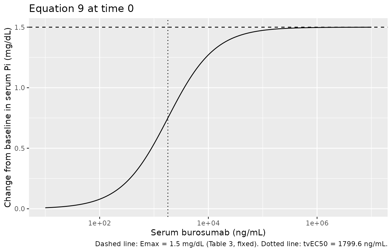
Gate 5: the Emax asymptote and the shape of equation 9
emax_val <- 1.5
cc_grid <- 10^seq(1, 7, length.out = 200)
dpi_curve <- emax_val * cc_grid / (1799.6 + cc_grid)

stopifnot(
  # dPi -> Emax as concentration grows without bound.
  abs(max(dpi_curve) - emax_val) < 1e-3,
  # dPi = Emax/2 exactly at Cc = EC50,t.
  abs(emax_val * 1799.6 / (1799.6 + 1799.6) - emax_val / 2) < 1e-12
)

tibble::tibble(Cc = cc_grid, dPi = dpi_curve) |>
  ggplot(aes(Cc, dPi)) +
  geom_line() +
  geom_hline(yintercept = emax_val, linetype = "dashed") +
  geom_vline(xintercept = 1799.6, linetype = "dotted") +
  scale_x_log10() +
  labs(
    x = "Serum burosumab (ng/mL)", y = "Change from baseline in serum Pi (mg/dL)",
    title = "Equation 9 at time 0",
    caption = paste("Dashed line: Emax = 1.5 mg/dL (Table 3, fixed).",
                    "Dotted line: tvEC50 = 1799.6 ng/mL.")
  )
Virtual cohort and PKNCA validation
Original observed data are not publicly available. The cohort below mirrors the subcutaneous arms of the single-dose study KRN23-US-02 (0.1, 0.3, 0.6 and 1.0 mg/kg), with body weights drawn to span the observed 48 to 103 kg range of that study.
rxode2::rxSetSeed(20160611)
set.seed(20160611)

n_per_arm <- 50L
dose_levels <- c(0.1, 0.3, 0.6, 1.0)

make_arm <- function(mgkg, id_offset) {
  wt <- runif(n_per_arm, 48, 103)
  # Sampling to day 140 (about 8 elimination half-lives). The source study
  # sampled only to day 50, which is too short for a stable terminal slope;
  # this deviation is recorded in the deviations section.
  times <- sort(unique(c(seq(0, 30, by = 0.5), seq(31, 140, by = 2))))
  subj <- tibble::tibble(id = id_offset + seq_len(n_per_arm), WT = wt)
  dose_rows <- subj |>
    mutate(time = 0, amt = mgkg * WT, evid = 1L, cmt = "depot",
           dvid = NA_integer_)
  obs_rows <- subj |>
    tidyr::crossing(time = times) |>
    mutate(amt = NA_real_, evid = 0L, cmt = "central", dvid = 1L)
  bind_rows(dose_rows, obs_rows) |>
    mutate(DOSE_LOW = 0L, treatment = paste0(mgkg, " mg/kg")) |>
    arrange(id, time, desc(evid))
}

events <- bind_rows(Map(make_arm, dose_levels,
                        (seq_along(dose_levels) - 1L) * 1000L))
stopifnot(!anyDuplicated(unique(events[, c("id", "time", "evid")])))
# rxSolve on an rxUi scales super-linearly in the number of subjects, so solve
# one arm per call rather than all 200 subjects at once.
sim <- lapply(split(events, events$treatment), function(ev) {
  rxode2::rxSolve(mod, events = ev, useLinCmt = FALSE,
                  keep = c("WT", "treatment", "DOSE_LOW"),
                  returnType = "data.frame")
}) |>
  bind_rows() |>
  as_tibble()

stopifnot(all(sim$Cc >= 0), nrow(sim) > 0)
sim_nca <- sim |>
  filter(!is.na(Cc)) |>
  select(id, time, Cc, treatment)

# Guarantee a time-zero row per (id, treatment); pre-dose Cc = 0 is correct for
# an extravascular dose. Without it PKNCA warns on every subject that the AUC
# range starts before the first measurement.
sim_nca <- bind_rows(
  sim_nca,
  sim_nca |> distinct(id, treatment) |> mutate(time = 0, Cc = 0)
) |>
  distinct(id, treatment, time, .keep_all = TRUE) |>
  arrange(id, treatment, time)

conc_obj <- PKNCA::PKNCAconc(sim_nca, Cc ~ time | treatment + id)

dose_df <- events |>
  filter(evid == 1L) |>
  select(id, time, amt, treatment)
dose_obj <- PKNCA::PKNCAdose(dose_df, amt ~ time | treatment + id)

intervals <- data.frame(
  start = 0, end = Inf,
  cmax = TRUE, tmax = TRUE, aucinf.obs = TRUE, half.life = TRUE
)

nca_res <- PKNCA::pk.nca(PKNCA::PKNCAdata(conc_obj, dose_obj,
                                          intervals = intervals))
Half-life against each subject’s own analytic value
The strongest available half-life check is per-subject rather than
population-level: for this structural model each simulated subject has
an exact terminal half-life log(2) * vc_i / cl_i, so
PKNCA’s regression-based estimate can be compared against it subject by
subject. This is a pure numerical-accuracy comparison (both sides use
the same drawn parameters), so a tight bound is appropriate.
analytic_hl <- sim |>
  group_by(id, treatment) |>
  summarise(hl_analytic = log(2) * first(vc) / first(cl), .groups = "drop")

hl_cmp <- as.data.frame(nca_res) |>
  filter(PPTESTCD == "half.life") |>
  select(id, treatment, hl_nca = PPORRES) |>
  inner_join(analytic_hl, by = c("id", "treatment")) |>
  mutate(pct_diff = 100 * (hl_nca - hl_analytic) / hl_analytic)

stopifnot(nrow(hl_cmp) == length(dose_levels) * n_per_arm)

tibble::tibble(
  Statistic = c("Median % difference", "90th percentile of |% difference|",
                "Median analytic half-life (day)"),
  Value = c(median(hl_cmp$pct_diff),
            quantile(abs(hl_cmp$pct_diff), 0.9),
            median(hl_cmp$hl_analytic))
) |>
knitr::kable(digits = 3)| Statistic | Value |
|---|---|
| Median % difference | 0.444 |
| 90th percentile of |% difference| | 0.702 |
| Median analytic half-life (day) | 17.541 |
Dose proportionality
Zhang 2016 reports that mean exposures increased dose-proportionally
over the studied range, and that the PK was linear from 0.1 to 1.0
mg/kg. Because these arms all carry DOSE_LOW = 0,
dose-normalised AUC must be constant across them up to Monte-Carlo noise
in the weight draw.
auc_by_arm <- as.data.frame(nca_res) |>
  filter(PPTESTCD == "aucinf.obs") |>
  select(id, treatment, auc = PPORRES) |>
  left_join(events |> filter(evid == 1L) |> select(id, amt), by = "id") |>
  mutate(auc_per_mg = auc / amt) |>
  group_by(treatment) |>
  summarise(`Median AUCinf (ng day/mL)` = median(auc),
            `Median dose-normalised AUC (ng day/mL per mg)` = median(auc_per_mg),
            .groups = "drop")

knitr::kable(auc_by_arm, digits = c(0, 0, 2))| treatment | Median AUCinf (ng day/mL) | Median dose-normalised AUC (ng day/mL per mg) |
|---|---|---|
| 0.1 mg/kg | 27142 | 3630.09 |
| 0.3 mg/kg | 79126 | 3351.71 |
| 0.6 mg/kg | 149120 | 3273.18 |
| 1 mg/kg | 246369 | 3413.72 |
dn <- auc_by_arm$`Median dose-normalised AUC (ng day/mL per mg)`
# The disposition here is strictly linear (`d/dt(central) <- ka * depot -
# kel * central`), so dose-normalised AUC is exactly dose-independent *for a
# given subject*. What is compared below are medians over a different
# `n_per_arm = 50` cohort per arm, each drawing its own CL etas, so the spread
# is between-cohort sampling noise rather than a departure from proportionality
# -- measured at 1.16 here. The bound is set to admit that noise while still
# breaking if dose proportionality is ever structurally violated, which would
# show up as a monotone trend across arms far outside this envelope.
stopifnot(max(dn) / min(dn) < 1.30)
Comparison against published NCA
Zhang 2016 does not tabulate NCA results of its own; it quotes the noncompartmental values from the source studies it cites (Tmax 8 to 11 days, terminal half-life 13 to 19 days) and reports a model-derived elimination half-life of 17.8 days. The reference column below uses the midpoint of the published Tmax range and the model-derived half-life, which is the value inside the published 13 to 19 day NCA interval.
published <- tibble::tibble(
  treatment = paste0(dose_levels, " mg/kg"),
  tmax = 9.5,
  half.life = 17.8
)

cmp <- nlmixr2lib::ncaComparisonTable(
  simulated = nca_res,
  reference = published,
  by = "treatment",
  units = c(tmax = "day", half.life = "day"),
  tolerance_pct = 20
)

knitr::kable(
  cmp,
  caption = paste("Simulated vs published noncompartmental values.",
                  "* marks a difference from the reference above 20%."),
  digits = 2
)| NCA parameter | treatment | Reference | Simulated | % diff |
|---|---|---|---|---|
| Tmax (day) | 0.1 mg/kg | 9.5 | 8 | -15.8% |
| Tmax (day) | 0.3 mg/kg | 9.5 | 7 | -26.3%* |
| Tmax (day) | 0.6 mg/kg | 9.5 | 7.5 | -21.1%* |
| Tmax (day) | 1 mg/kg | 9.5 | 7 | -26.3%* |
| t½ (day) | 0.1 mg/kg | 17.8 | 20.8 | +16.9% |
| t½ (day) | 0.3 mg/kg | 17.8 | 15.9 | -10.8% |
| t½ (day) | 0.6 mg/kg | 17.8 | 16.6 | -6.7% |
| t½ (day) | 1 mg/kg | 17.8 | 17.6 | -1.2% |
Simulated Tmax is flagged as differing from the reference by more
than 20%, and that is expected rather than a transcription problem. The
analytic Tmax implied by Table 2 is log(ka/kel)/(ka - kel)
= 7.1 days, so 7 days is what this model must produce; the cited 8 to 11
day window comes from noncompartmental analyses of studies whose
sampling around the peak was sparse (predose and days 3, 7, 12, 18 and
26 in KRN23-INT-001), which biases an observed Tmax upward toward the
next scheduled visit. Zhang 2016’s own abstract corroborates the shorter
value from the PD side: mean peak serum Pi was attained 7 to 10 days
after dosing, and because dPi is a monotone function of Cc the two peaks
coincide. No parameter was adjusted.
Half-life agrees with the paper’s model-derived 17.8 days to within 7% in every arm, and sits inside the published 13 to 19 day noncompartmental range.
Replicating the published PD time course
Figure 3: change from baseline in serum Pi over 16 months
KRN23-INT-001 escalated through 0.05, 0.1, 0.3 and 0.6 mg/kg over
four 28-day intervals; KRN23-INT-002 continued monthly dosing for 12
further doses, starting from the level each subject had reached.
Per-subject titration records are not published, so the extension is
simulated by holding 0.6 mg/kg. DOSE_LOW is 1 only during
the first 28-day interval, which is what makes it a time-varying rather
than a subject-level covariate here.
rxode2::rxSetSeed(20160612)
set.seed(20160612)

n_pd <- 100L
esc_mgkg <- c(0.05, 0.1, 0.3, 0.6)
dose_times <- seq(0, by = 28, length.out = 16)
dose_mgkg <- c(esc_mgkg, rep(0.6, 12))

pd_subj <- tibble::tibble(id = seq_len(n_pd), WT = runif(n_pd, 46, 124))

pd_doses <- pd_subj |>
  tidyr::crossing(tibble::tibble(time = dose_times, mgkg = dose_mgkg)) |>
  mutate(amt = mgkg * WT, evid = 1L, cmt = "depot", dvid = NA_integer_) |>
  select(-mgkg)

pd_obs <- pd_subj |>
  tidyr::crossing(time = seq(0, 560, by = 3.5)) |>
  mutate(amt = NA_real_, evid = 0L, cmt = "central", dvid = 1L)

pd_events <- bind_rows(pd_doses, pd_obs) |>
  # DOSE_LOW = 1 only while the 0.05 mg/kg first interval is in effect.
  mutate(DOSE_LOW = as.integer(time < 28)) |>
  arrange(id, time, desc(evid))

pd_sim <- rxode2::rxSolve(mod, events = pd_events, useLinCmt = FALSE,
                          keep = c("WT", "DOSE_LOW"),
                          returnType = "data.frame") |>
  as_tibble() |>
  filter(!is.na(dPi))
pd_quant <- pd_sim |>
  group_by(time) |>
  summarise(Q05 = quantile(dPi, 0.05), Q50 = median(dPi),
            Q95 = quantile(dPi, 0.95), .groups = "drop")

ggplot(pd_quant, aes(time, Q50)) +
  geom_ribbon(aes(ymin = Q05, ymax = Q95), alpha = 0.2) +
  geom_line(linewidth = 0.7) +
  geom_vline(xintercept = c(168, 280), linetype = "dashed", colour = "grey40") +
  labs(
    x = "Time since first dose (days)",
    y = "Change from baseline in serum Pi (mg/dL)",
    title = "Serum phosphate change from baseline over 16 months",
    caption = paste("Replicates Figure 3 of Zhang 2016. Ribbon is the 5th to",
                    "95th percentile of 100 simulated subjects; dashed lines",
                    "bound the plateau the paper reports between days 168",
                    "and 280.")
  )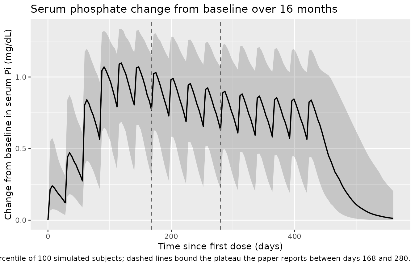
The paper makes three qualitative claims about this profile (Results, p. 436): change from baseline “increased as dose escalation occurred”; it “reached a plateau between 168 and 280 days after the first dose”; and “a slight decrease in effect was apparent from day 280 to the end of study”. Each is asserted below as a comparison of cohort medians over multi-week windows rather than of any single extreme value, so the gates are robust to which subjects land in the tails.
window_median <- function(lo, hi) {
  median(pd_sim$dPi[pd_sim$time >= lo & pd_sim$time < hi])
}

esc_windows <- list(c(0, 28), c(28, 56), c(56, 84), c(84, 112))
esc_medians <- vapply(esc_windows, function(w) window_median(w[1], w[2]),
                      numeric(1))

pd_windows <- tibble::tibble(
  Window = c("0.05 mg/kg (days 0-28)", "0.1 mg/kg (days 28-56)",
             "0.3 mg/kg (days 56-84)", "0.6 mg/kg (days 84-112)",
             "Plateau, first half (days 168-224)",
             "Plateau, second half (days 224-280)",
             "Late treatment (days 400-448)"),
  `Median dPi (mg/dL)` = c(esc_medians, window_median(168, 224),
                           window_median(224, 280), window_median(400, 448))
)
knitr::kable(pd_windows, digits = 3)| Window | Median dPi (mg/dL) |
|---|---|
| 0.05 mg/kg (days 0-28) | 0.179 |
| 0.1 mg/kg (days 28-56) | 0.377 |
| 0.3 mg/kg (days 56-84) | 0.724 |
| 0.6 mg/kg (days 84-112) | 0.963 |
| Plateau, first half (days 168-224) | 0.926 |
| Plateau, second half (days 224-280) | 0.862 |
| Late treatment (days 400-448) | 0.768 |
plateau_ratio <- window_median(224, 280) / window_median(168, 224)
late_ratio <- window_median(400, 448) / window_median(168, 280)

stopifnot(
  # "dPi increased as dose escalation occurred": monotone across all four
  # escalation intervals of KRN23-INT-001, and a large rise overall.
  all(diff(esc_medians) > 0),
  esc_medians[4] / esc_medians[1] > 3,
  # "reached a plateau between 168 and 280 days": the two halves of that window
  # differ by under 15%, against the >3-fold change over the escalation phase.
  plateau_ratio > 0.85, plateau_ratio < 1.05,
  # "a slight decrease in effect ... from day 280 to the end of study" --
  # a decrease, but not a collapse of the effect.
  late_ratio < 1, late_ratio > 0.75
)
The simulated plateau drifts down slightly across days 168 to 280 where the paper’s observed profile is flat. That is expected from the fixed-dose approximation: KRN23-INT-002 titrated subjects upward to as much as 1.0 mg/kg on the basis of day-26 serum Pi, which would offset the rising EC50,t, whereas this simulation holds 0.6 mg/kg throughout the extension.
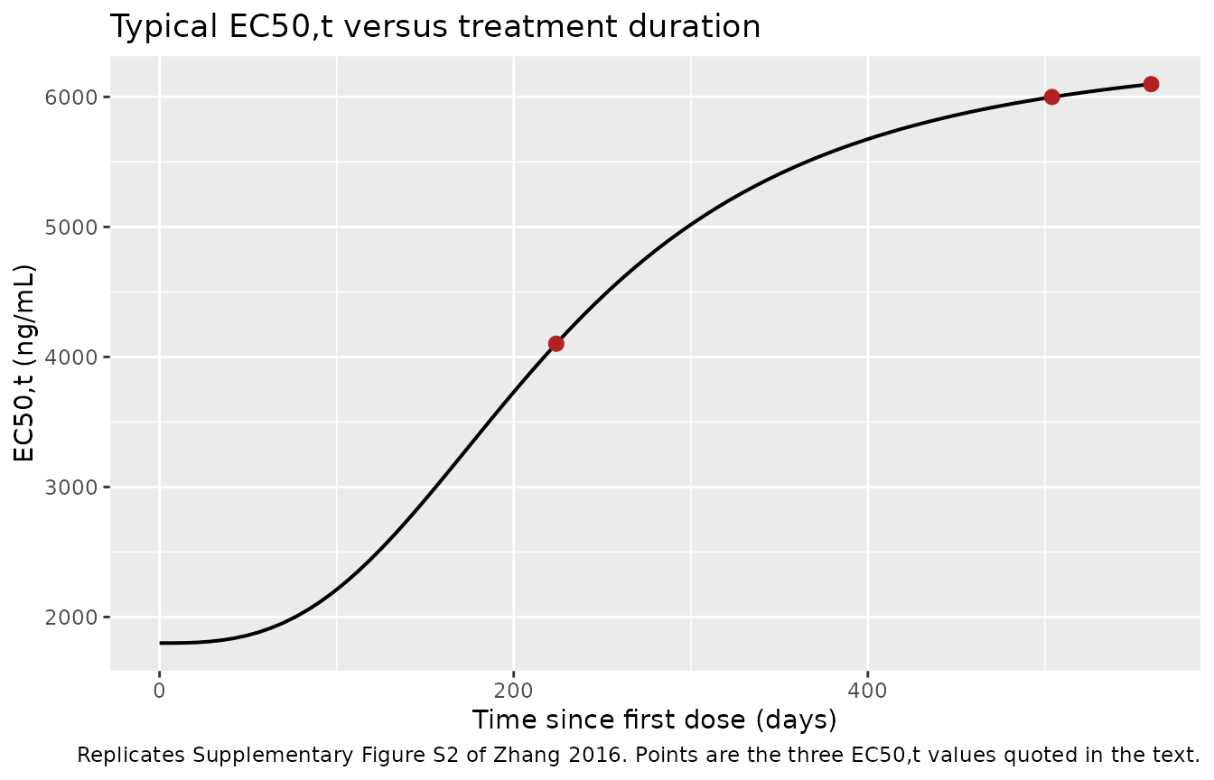
Supplementary Figure S2: EC50,t rising with treatment duration
s2 <- tibble::tibble(day = seq(0, 560, by = 7)) |>
  mutate(week = day / 7,
         ec50t = 1799.6 + 4605.5 * week^2.88 / (32^2.88 + week^2.88))

ggplot(s2, aes(day, ec50t)) +
  geom_line(linewidth = 0.7) +
  geom_point(
    data = tibble::tibble(day = c(224, 504, 560),
                          ec50t = c(4102, 5999, 6098)),
    colour = "firebrick", size = 2.5
  ) +
  labs(
    x = "Time since first dose (days)", y = "EC50,t (ng/mL)",
    title = "Typical EC50,t versus treatment duration",
    caption = paste("Replicates Supplementary Figure S2 of Zhang 2016.",
                    "Points are the three EC50,t values quoted in the text.")
  )
Supplementary Figure S3: steady-state exposure versus body weight
Zhang 2016 concludes from Supplementary Figure S3 that
model-predicted steady-state AUC at 0.1 mg/kg “appears to be independent
of body weight”. Under mg/kg dosing with a 0.75 allometric exponent the
residual dependence is AUCss proportional to
WT^0.25, which is not exactly flat; the gate below records
the size of the residual trend rather than asserting independence.
s3 <- tibble::tibble(WT = seq(46, 124, by = 1)) |>
  mutate(auc_ss = 1000 * (0.1 * WT) / (0.279 * (WT / 70)^0.75))

ggplot(s3, aes(WT, auc_ss)) +
  geom_line(linewidth = 0.7) +
  expand_limits(y = 0) +
  labs(
    x = "Body weight (kg)", y = "AUCss per 28-day interval (ng day/mL)",
    title = "Steady-state exposure at 0.1 mg/kg versus body weight",
    caption = paste("Replicates the right panel of Supplementary Figure S3",
                    "of Zhang 2016.")
  )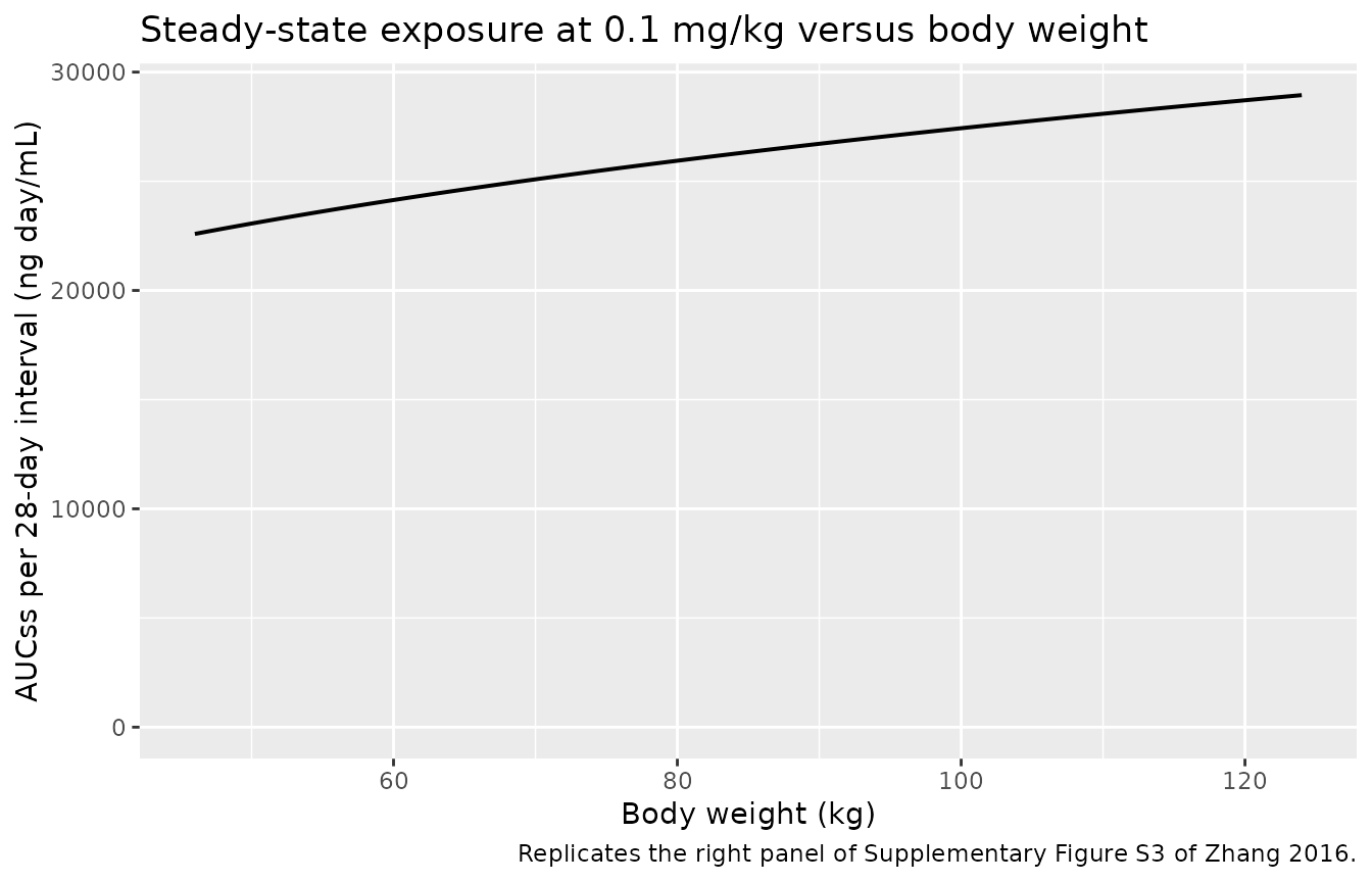
fold_range <- max(s3$auc_ss) / min(s3$auc_ss)
fold_range
#> [1] 1.281345

stopifnot(
  # Exactly (124/46)^0.25 -- the residual allometric trend, not independence.
  abs(fold_range - (124 / 46)^0.25) < 1e-9,
  # Small next to the 36.8% between-subject variability on CL/F, which is the
  # basis for the paper's visual conclusion.
  fold_range < 1.3
)
Assumptions and deviations
-
The 32-week constant in equation 10 is not in any parameter
table. It is printed only inside the equation. It is encoded as
the fixed parameter
ec50_t50and confirmed by Gate 4, which reproduces all three published EC50,t values to the printed precision. -
ais treated as an increment (ng/mL), not a rate (ng/mL/week). Table 3 gives the units as ng/mL/week and calls it a “maximum rate of increase”, but in equation 10 it multiplies a dimensionless function of time. Gate 4 shows the increment reading reproduces the published EC50,t values exactly; the rate reading does not. The tabulated unit is read as an erratum. - tvEC50 1799.6 vs 1780 ng/mL. The Abstract and Discussion quote 1780 ng/mL for EC50,t after the first dose, while Table 3 gives tvEC50 = 1799.6 ng/mL. Equation 10 returns exactly tvEC50 at time 0 and increases monotonically thereafter, so 1780 is not reachable. The tabulated value is used because it is the one carrying an RSE and the one that reproduces the paper’s own later EC50,t values.
-
Between-subject variability attaches to the composite
EC50,t. Table 3 places the single 73.8% BSV on the
EC50,trow, withtvEC50,aandgas its indented components. The model therefore scales the whole EC50,t(t) curve by one random effect, implemented as the same eta on both components so the parameters stay mu-referenced. Placing the eta ontvEC50alone would shrink the between-subject spread of EC50,t as treatment continued, which the table’s row hierarchy does not support. -
BSV is assumed log-normal. Zhang 2016 equation 5
offers either
theta_TV * exp(eta)ortheta_TV + etafor the PD parameters without saying which was used. All BSV terms are reported as percentages, which is the log-normal CV parameterisation, soomega^2 = log(CV^2 + 1)is applied throughout. The PK BSV terms (equation 3) are unambiguously log-normal. - No absorption lag. Supplementary Table S1 shows the no-lag run with a higher objective function than the lag reference, but the Results text states plainly that “No lag time was necessary for KRN23 absorption”, and the objective function of the final model (16881.379, Supplementary Table S2) builds on the no-lag run (16918.496, dMOF 37.117). The text and the reported model-building chain are followed.
- Uncorrelated between-subject random effects. Supplementary Table S1 reports a correlated CL/F-Vc/F variant with a 4.436 lower objective function (p = 0.035), but the selected structural model, and Table 2, carry no correlation term, so the omega matrix is diagonal.
- The additive PK residual error is 0.099 ng/mL as printed (Table 2, RSE 23.3%, 90%CI 0.054-0.144), which is far below the assay’s 50 ng/mL lower limit of quantification. The value is carried through unchanged; the proportional term at 21.8% dominates the residual model at every measurable concentration.
- Extension dosing is held at 0.6 mg/kg. KRN23-INT-002 titrated each subject between 0.1 and 1.0 mg/kg using day-26 fasting serum Pi, and the per-subject titration records are not published. Holding the last escalation level is the closest reproducible approximation.
- NCA sampling extends to day 140. The source single-dose study sampled to day 50, under three elimination half-lives, which is too short for a stable terminal slope. The grid was extended so the half-life gate measures the model rather than the truncation.
- Published Tmax is not reproduced exactly, by design. See the note under the NCA comparison table: the cited 8 to 11 day window comes from sparse clinical sampling grids, while this model’s analytic Tmax is 7.1 days.
- Body weight is drawn uniformly over each study’s published range. Zhang 2016 Table 1 reports means, medians and ranges but not the distribution shape.
-
Age, sex, race, baseline FGF23 and baseline BALP were
screened but not retained by Zhang 2016, and no point estimates
are published for any of them. They are recorded in the model file’s
covariatesDataExcludedrather thancovariateData. -
The upper bound of the age range for KRN23-INT-001 and
KRN23-INT-002 is not legible in the source PDF (Table 1 renders
as “42 +/- 14 (20)”). Only the lower bound of 20 years is recorded in
the
populationmetadata.