Ciprofloxacin (Abdulla 2020)
Source:vignettes/articles/Abdulla_2020_ciprofloxacin.Rmd
Abdulla_2020_ciprofloxacin.RmdModel and source
- Citation: Abdulla A, Rogouti O, Hunfeld NGM, Endeman H, Dijkstra A, van Gelder T, Muller AE, de Winter BCM, Koch BCP. Population pharmacokinetics and target attainment of ciprofloxacin in critically ill patients. Eur J Clin Pharmacol. 2020;76(7):957-967. doi:10.1007/s00228-020-02873-5
- Description: Two-compartment population PK model for intravenous ciprofloxacin in adult ICU patients (Abdulla 2020). Linear elimination from the central compartment, IIV on CL and Vc, and a combined additive + proportional residual error. The model was fitted to protein-binding-corrected (unbound) plasma concentrations, so the observation Cc = central / vc is the UNBOUND concentration; total plasma ciprofloxacin is reconstructed as Ctot = Cc / fu with the paper’s assumed 30% plasma protein binding (fu = 0.7). Serum creatinine, eGFR, albumin, BMI, weight, sex, renal replacement therapy and age were screened but none was retained.
- Article: https://doi.org/10.1007/s00228-020-02873-5 (open access)
Population
Abdulla et al. (2020) enrolled 42 adult ICU patients treated with
intravenous ciprofloxacin at the Erasmus Medical Centre and Maasstad
Hospital, Rotterdam (EXPAT study, 2016). 25 were male and 17 female;
median age 65.5 years (IQR 56-71), weight 80 kg (IQR 64-90), BMI 26
kg/m^2, APACHE II 22 and SOFA 13. Median eGFR (MDRD) was 58.5
mL/min/1.73 m^2 (IQR 32-101) and 10 patients (23.8%) were on continuous
venovenous haemofiltration. Patients received 400 mg q24h (n = 3), q12h
(n = 25) or q8h (n = 14) as 30-60 min infusions and were sampled on day
2 of therapy (pre-dose, 15-30 min after the end of the infusion, 1 h and
3 h after the infusion and before the next dose), giving 204
concentrations. Demographics are in the source Table 1 and in
readModelDb("Abdulla_2020_ciprofloxacin")$population.
Serum creatinine, eGFR, albumin, BMI, weight, sex, renal replacement
therapy and age were screened; none was retained, so the final model
carries no covariate effects. The screened covariates are recorded in
the model’s covariatesDataExcluded metadata.
Source trace
| Equation / parameter | Value | Source location |
|---|---|---|
lcl (CL) |
log(25.4 L/h) | Table 2, final model |
lvc (Vc) |
log(91.1 L) | Table 2, final model |
lvp (Vp) |
log(164 L) | Table 2, final model |
lq (Q) |
log(91.9 L/h) | Table 2, final model |
fu |
fixed 0.7 | Methods ‘Blood sampling and assays’ (average PPB 30%, fAUC = AUC x 0.7) |
etalcl |
0.3782 | Table 2, IIV CL 67.8% -> log(1 + 0.678^2) |
etalvc |
0.2312 | Table 2, IIV Vc 51.0% -> log(1 + 0.510^2) |
propSd |
0.153 | Table 2, proportional residual 15.3% |
addSd |
0.143 mg/L | Table 2, additive residual ‘14.3’ (read as 0.143 mg/L; see Assumptions) |
| Two-compartment model, IV infusion | n/a | Methods ‘Structural model’; Results ‘Final model’ |
| Combined additive + proportional error | n/a | Methods ‘Structural model’; Results ‘Final model’ |
| No covariates | n/a | Results ‘Covariate analysis’ |
Cc = unbound, Ctot = Cc / fu
|
n/a | Methods PPB correction; confirmed by the AUC checks below |
Virtual cohorts
Two sets of cohorts are simulated, 200 virtual patients per arm:
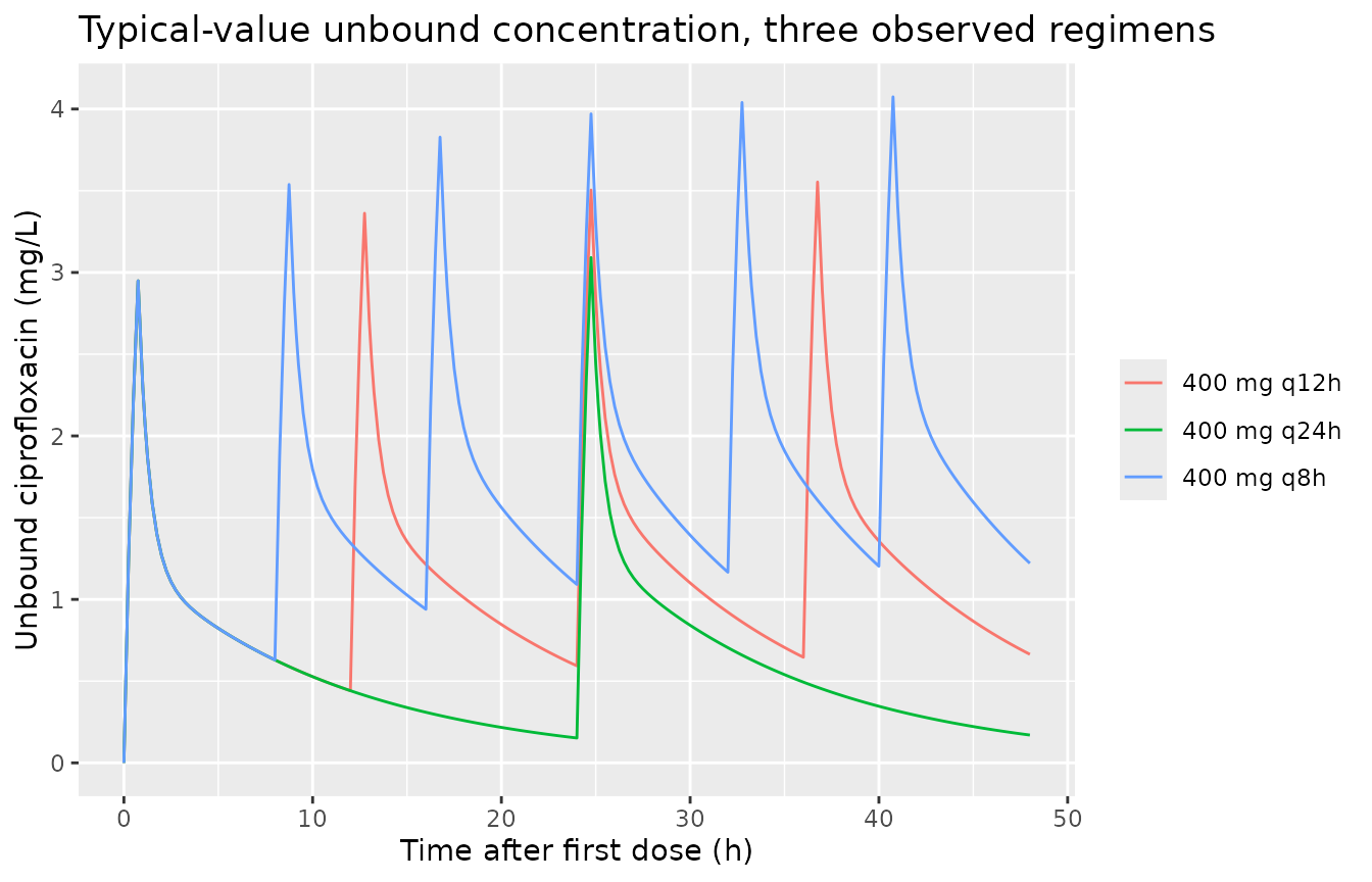
- The three observed dose groups (400 mg q24h, q12h and q8h, 45-min infusions – the midpoint of the reported 30-60 min), observed densely over day 2 (24-48 h) to compare with the reported day-2 exposure metrics.
- The five regimens of the paper’s Monte Carlo analysis (Fig. 4): 400 mg q12h, q8h and q6h, and 600 mg q12h and q8h.
n_per_arm <- 200L
tinf <- 0.75

make_arm <- function(arm, dose, tau, id_offset, t_end = 48) {
  ids <- id_offset + seq_len(n_per_arm)
  dose_times <- seq(0, t_end - tau, by = tau)
  obs_times <- sort(unique(c(
    seq(0, t_end, by = 0.25),
    dose_times + tinf,
    dose_times + tinf + 0.375
  )))
  dose_rows <- expand.grid(id = ids, time = dose_times) |>
    dplyr::mutate(amt = dose, rate = dose / tinf, evid = 1L, cmt = "central")
  obs_rows <- expand.grid(id = ids, time = obs_times) |>
    dplyr::mutate(amt = NA_real_, rate = NA_real_, evid = 0L, cmt = "central")
  dplyr::bind_rows(dose_rows, obs_rows) |>
    dplyr::mutate(arm = arm, daily_dose = dose * 24 / tau) |>
    dplyr::arrange(id, time, -evid)
}

obs_groups <- c("400 mg q24h" = 24, "400 mg q12h" = 12, "400 mg q8h" = 8)
events_obs <- dplyr::bind_rows(lapply(seq_along(obs_groups), function(i) {
  make_arm(names(obs_groups)[i], 400, obs_groups[[i]], id_offset = (i - 1) * 1000L)
}))
Simulation
mod <- rxode2::rxode(readModelDb("Abdulla_2020_ciprofloxacin"))
#> ℹ parameter labels from comments will be replaced by 'label()'
rxode2::rxSetSeed(20200419)
sim_obs <- rxode2::rxSolve(
  mod,
  events = events_obs,
  keep = c("arm", "daily_dose")
) |>
  as.data.frame()
Typical profile
mod_typ <- mod |> rxode2::zeroRe()
sim_typ <- rxode2::rxSolve(
  mod_typ,
  events = events_obs |> dplyr::filter(id %in% c(1L, 1001L, 2001L)),
  keep = "arm"
) |>
  as.data.frame()
#> ℹ omega/sigma items treated as zero: 'etalcl', 'etalvc'
#> Warning: multi-subject simulation without without 'omega'

ggplot(sim_typ, aes(time, Cc, colour = arm)) +
  geom_line() +
  labs(
    x = "Time after first dose (h)",
    y = "Unbound ciprofloxacin (mg/L)",
    colour = NULL,
    title = "Typical-value unbound concentration, three observed regimens"
  )
Day-2 VPC
Figure 3 of the source is a VPC of all dosing groups against time after dose. The plot below shows the simulated 5th, 50th and 95th percentiles over the day-2 q12h interval (24-36 h), the dominant regimen (25 of 42 patients).
# Replicates Figure 3 of Abdulla 2020 (VPC of the final model; q12h interval).
vpc <- sim_obs |>
  dplyr::filter(arm == "400 mg q12h", time >= 24, time <= 36) |>
  dplyr::mutate(tad = time - 24) |>
  dplyr::group_by(tad) |>
  dplyr::summarise(
    p05 = quantile(sim, 0.05),
    p50 = quantile(sim, 0.50),
    p95 = quantile(sim, 0.95),
    .groups = "drop"
  )

ggplot(vpc, aes(tad, p50)) +
  geom_ribbon(aes(ymin = p05, ymax = p95), fill = "steelblue", alpha = 0.25) +
  geom_line(colour = "firebrick", linewidth = 0.9) +
  labs(
    x = "Time after dose (h)",
    y = "Ciprofloxacin concentration (mg/L)",
    caption = "Replicates Figure 3 of Abdulla 2020 (5th / 50th / 95th percentiles, with residual error)."
  )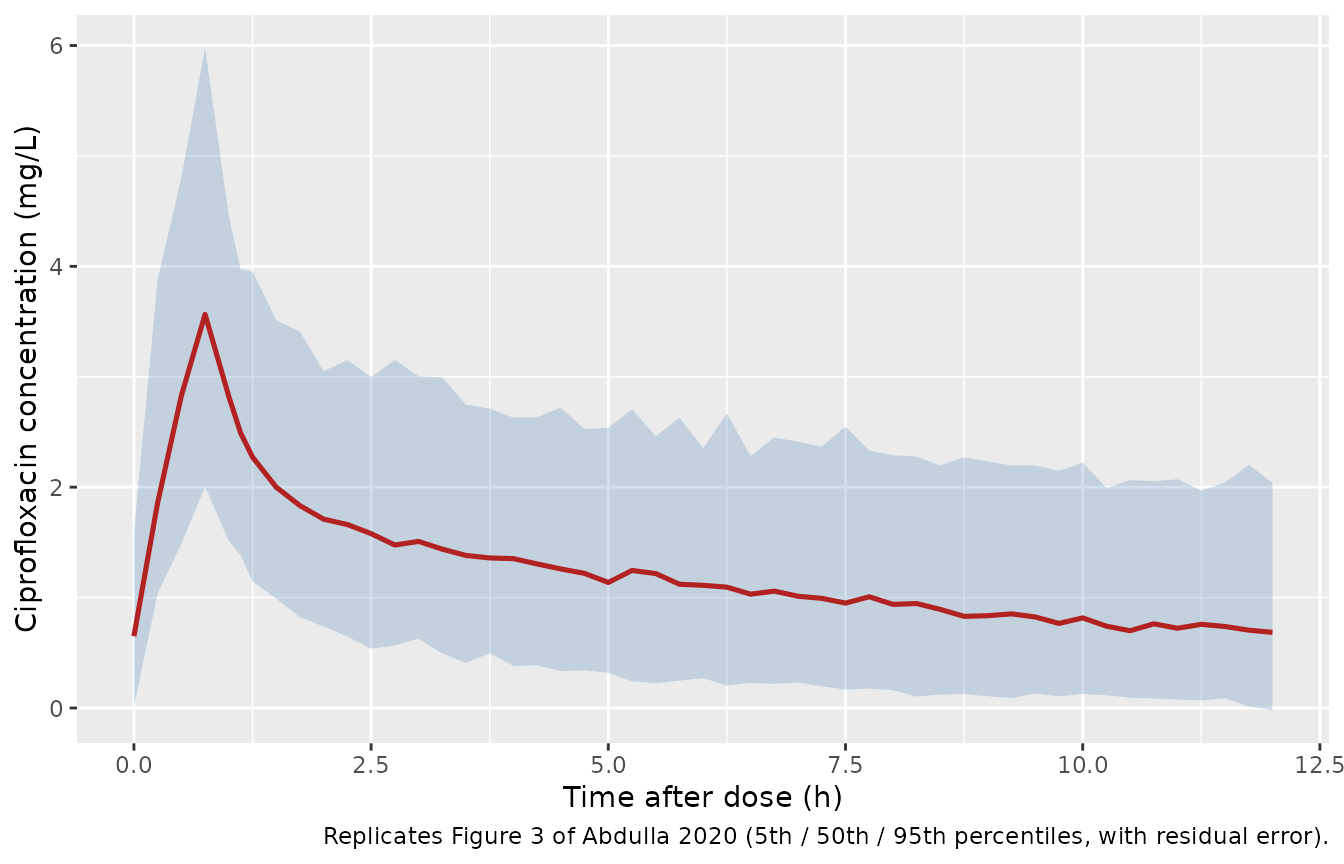
The simulated median peaks at about 3.6 mg/L at the end of the infusion, is about 1.4 mg/L at 4 h and falls to about 0.7 mg/L by 12 h. The published VPC pools all three regimens (its time axis ends near 8 h, the q8h interval) and shows a median of about 3 mg/L at the peak sample and about 1.3 mg/L over 3-7 h, the same level and shape.
PKNCA validation
PKNCA is run twice over day 2, the sampling day of the study.
Cc is the unbound concentration, so its AUC and Cmax are
directly the paper’s fAUC0-24 and fCmax.
- AUC0-24 uses the dense 15-min grid over 24-48 h.
- Cmax uses the study’s own sampling design on the first day-2 dose: pre-dose, 22.5 min after the end of the infusion (midpoint of the stated 15-30 min), 1 h and 3 h after the infusion, and pre-next-dose. The published fCmax is the peak sample, which is lower than the true end-of-infusion peak; the dense-grid Cmax is shown alongside for reference.
dose_nca <- events_obs |>
  dplyr::filter(evid == 1) |>
  dplyr::select(id, time, amt, arm)
dose_obj <- PKNCA::PKNCAdose(dose_nca, amt ~ time | arm + id)

conc_dense <- sim_obs |>
  dplyr::filter(!is.na(Cc)) |>
  dplyr::select(id, time, Cc, arm)
nca_dense <- PKNCA::pk.nca(PKNCA::PKNCAdata(
  PKNCA::PKNCAconc(conc_dense, Cc ~ time | arm + id),
  dose_obj,
  intervals = data.frame(start = 24, end = 48, cmax = TRUE, auclast = TRUE)
))

# Study sampling design on the first day-2 dose (24 h), per regimen.
tau_arm <- data.frame(arm = names(obs_groups), tau = unname(obs_groups))
design <- tidyr::expand_grid(
  tau_arm,
  tad = c(0, tinf + 0.375, tinf + 1, tinf + 3)
) |>
  dplyr::bind_rows(tau_arm |> dplyr::mutate(tad = tau)) |>
  dplyr::mutate(time = 24 + tad) |>
  dplyr::select(arm, time)
conc_sparse <- conc_dense |>
  dplyr::inner_join(design, by = c("arm", "time"))
stopifnot(nrow(conc_sparse) == 5L * n_per_arm * length(obs_groups))
nca_sparse <- PKNCA::pk.nca(PKNCA::PKNCAdata(
  PKNCA::PKNCAconc(conc_sparse, Cc ~ time | arm + id),
  dose_obj,
  intervals = data.frame(start = 24, end = 48, cmax = TRUE)
))

nca_df <- dplyr::bind_rows(
  as.data.frame(nca_dense$result) |>
    dplyr::mutate(design = "dense grid"),
  as.data.frame(nca_sparse$result) |>
    dplyr::mutate(design = "study sampling")
)

nca_summary <- nca_df |>
  dplyr::filter(PPTESTCD %in% c("cmax", "auclast")) |>
  dplyr::group_by(design, arm, PPTESTCD) |>
  dplyr::summarise(
    mean = mean(PPORRES),
    median = median(PPORRES),
    p05 = quantile(PPORRES, 0.05),
    p95 = quantile(PPORRES, 0.95),
    .groups = "drop"
  )

knitr::kable(
  nca_summary,
  digits = 2,
  caption = "Simulated day-2 unbound NCA by dose group and sampling design (mean, median, 5th and 95th percentiles)."
)| design | arm | PPTESTCD | mean | median | p05 | p95 |
|---|---|---|---|---|---|---|
| dense grid | 400 mg q12h | auclast | 33.70 | 31.64 | 12.06 | 64.05 |
| dense grid | 400 mg q12h | cmax | 3.78 | 3.65 | 2.20 | 5.93 |
| dense grid | 400 mg q24h | auclast | 15.98 | 14.40 | 5.38 | 33.62 |
| dense grid | 400 mg q24h | cmax | 3.01 | 2.93 | 1.66 | 4.46 |
| dense grid | 400 mg q8h | auclast | 47.70 | 44.89 | 17.75 | 93.00 |
| dense grid | 400 mg q8h | cmax | 4.13 | 3.95 | 2.25 | 6.52 |
| study sampling | 400 mg q12h | cmax | 2.57 | 2.52 | 1.43 | 3.94 |
| study sampling | 400 mg q24h | cmax | 2.03 | 1.98 | 1.26 | 2.93 |
| study sampling | 400 mg q8h | cmax | 2.92 | 2.86 | 1.61 | 4.64 |
Comparison against published values
The Results section reports the mean observed fCmax (3.10, 3.02 and 3.05 mg/L) and fAUC0-24 (26.6, 34.2 and 46.8 mg*h/L) for the q24h, q12h and q8h groups. The simulated group means (AUC from the dense grid, Cmax from the study sampling design) are compared against them below.
sim_means <- nca_summary |>
  dplyr::filter(
    (PPTESTCD == "auclast" & design == "dense grid") |
      (PPTESTCD == "cmax" & design == "study sampling")
  ) |>
  dplyr::select(arm, PPTESTCD, PPORRES = mean)

published <- data.frame(
  arm = names(obs_groups),
  cmax = c(3.10, 3.02, 3.05),
  auclast = c(26.6, 34.2, 46.8)
)

cmp <- nlmixr2lib::ncaComparisonTable(
  simulated = sim_means,
  reference = published,
  by = "arm",
  units = c(cmax = "mg/L", auclast = "mg*h/L"),
  tolerance_pct = 20
)
knitr::kable(
  cmp,
  caption = paste(
    "Simulated vs. published mean unbound day-2 exposure by dose group",
    "(Abdulla 2020 Results 'Pharmacokinetic parameters').",
    "* marks a difference above 20%."
  )
)| NCA parameter | arm | Reference | Simulated | % diff |
|---|---|---|---|---|
| Cmax (mg/L) | 400 mg q24h | 3.1 | 2.03 | -34.7%* |
| Cmax (mg/L) | 400 mg q12h | 3.02 | 2.57 | -14.7% |
| Cmax (mg/L) | 400 mg q8h | 3.05 | 2.92 | -4.4% |
| AUClast (mg*h/L) | 400 mg q24h | 26.6 | 16 | -39.9%* |
| AUClast (mg*h/L) | 400 mg q12h | 34.2 | 33.7 | -1.4% |
| AUClast (mg*h/L) | 400 mg q8h | 46.8 | 47.7 | +1.9% |
gate <- published |>
  tidyr::pivot_longer(-arm, names_to = "PPTESTCD", values_to = "ref") |>
  dplyr::left_join(sim_means, by = c("arm", "PPTESTCD")) |>
  dplyr::mutate(pct = 100 * (PPORRES - ref) / ref)

# The q12h and q8h groups (39 of 42 patients) carry the comparison; the q24h
# group (n = 3, median eGFR 28 mL/min/1.73 m^2) is reported but not gated.
# A cohort mean of 200 subjects has a Monte Carlo SE of about 5% for this IIV.
# AUC depends only on CL, so it gets the tighter bound; the sampled peak also
# depends on the infusion duration (30-60 min in the study, 45 min here), so
# it gets a wider one. Both still catch a total-vs-unbound mix-up, which would
# move every value by 1/0.7 = 43%.
main <- gate |> dplyr::filter(arm != "400 mg q24h")
stopifnot(
  nrow(main) == 4L,
  !anyNA(main$pct),
  all(abs(main$pct[main$PPTESTCD == "auclast"]) < 15),
  all(abs(main$pct[main$PPTESTCD == "cmax"]) < 25)
)
For the q12h and q8h groups the simulated mean fAUC0-24 agrees with the published mean within 2% and the sampled fCmax within 15%. The q24h group (three patients) has a markedly higher published fAUC0-24 than the model predicts: those three patients had a median eGFR of 28 mL/min/1.73 m^2 (they were presumably given once-daily dosing because of their renal impairment), whereas the model – which retained no renal covariate – predicts the population-typical clearance for them (their sampled fCmax is also under-predicted).
The overall Table 1 median fAUC0-24 of 29.9 mg*h/L (IQR 19.6-42.1) and median fCmax of 3.1 mg/L (IQR 2.4-4.0) pool the three groups and are consistent with the q12h row above.
Total vs unbound (why Cc is the unbound
concentration)
If the model had been fitted to total concentrations, the
model-predicted fAUC0-24 would be 0.7 x daily dose / CL. For 800 mg/day
that is 22.0 mgh/L at the typical CL, against the published q12h
mean of 34.2 and the overall median of 29.9; the unbound reading (daily
dose / CL = 31.5 mgh/L typical) matches both, and it also matches
the Fig. 4 curves below. The model is therefore packaged with
Cc as the unbound concentration and the total concentration
Ctot = Cc / fu.
Replicate Figure 4 (Monte Carlo fAUC0-24/MIC)
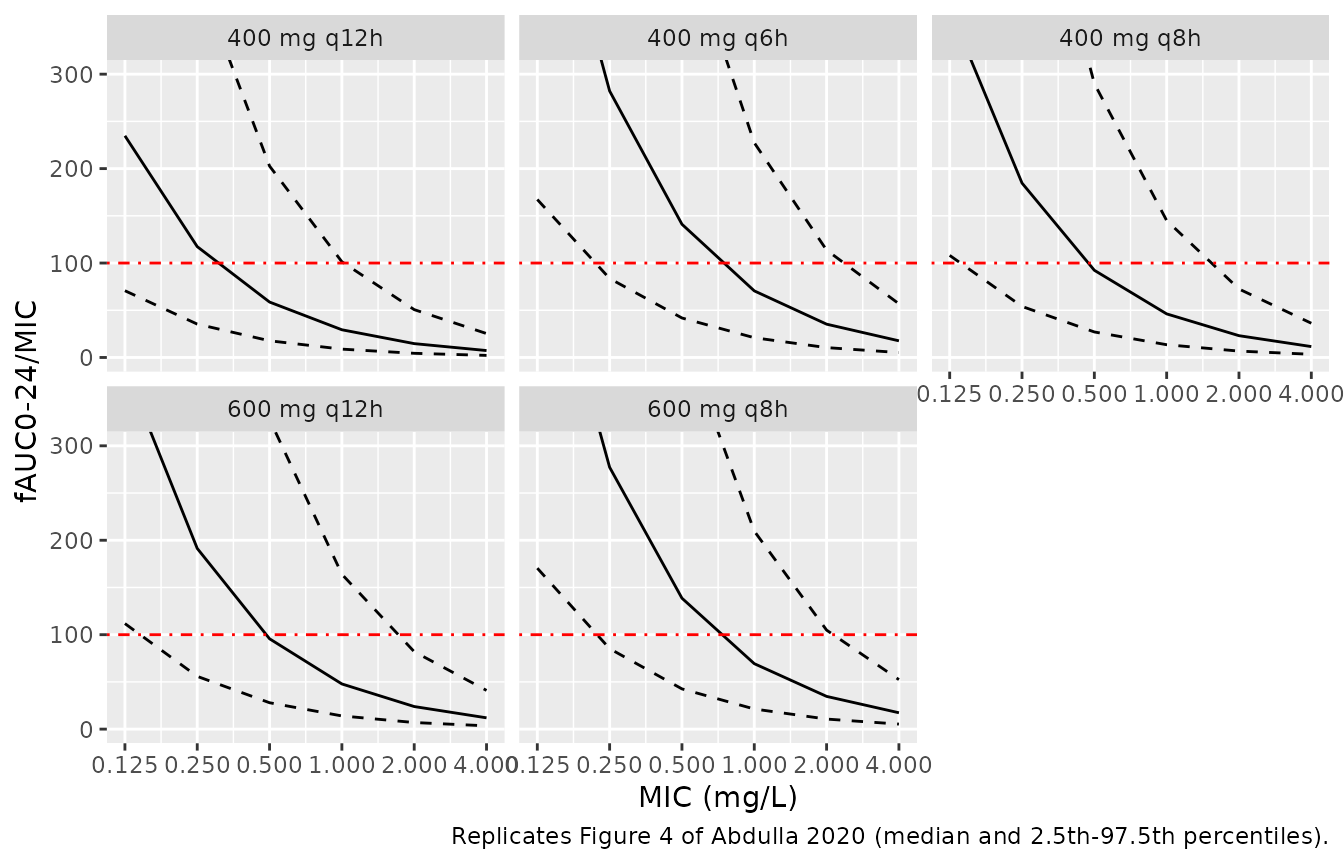
At steady state fAUC0-24 = daily dose / CL for each individual, so the distribution of fAUC0-24/MIC is set entirely by CL and its IIV. The paper’s Fig. 4 shows the ‘average’ fAUC0-24/MIC and its 95% and 99% confidence bounds against MIC for five regimens.
regimens <- data.frame(
  regimen = c("400 mg q12h", "400 mg q8h", "400 mg q6h", "600 mg q12h", "600 mg q8h"),
  daily_dose = c(800, 1200, 1600, 1200, 1800)
)
rxode2::rxSetSeed(20200420)
omega_cl <- mod$omega["etalcl", "etalcl"]
ind <- regimens[rep(seq_len(nrow(regimens)), each = n_per_arm), ] |>
  dplyr::mutate(cl = typ_cl * exp(rnorm(dplyr::n(), 0, sqrt(omega_cl))),
                fauc24 = daily_dose / cl)

mics <- c(0.125, 0.25, 0.5, 1, 2, 4)
fig4 <- tidyr::expand_grid(ind, mic = mics) |>
  dplyr::group_by(regimen, mic) |>
  dplyr::summarise(
    median = median(fauc24 / mic),
    lo = quantile(fauc24 / mic, 0.025),
    hi = quantile(fauc24 / mic, 0.975),
    pta = mean(fauc24 / mic >= 100),
    .groups = "drop"
  )

ggplot(fig4, aes(mic, median)) +
  geom_line() +
  geom_line(aes(y = lo), linetype = "dashed") +
  geom_line(aes(y = hi), linetype = "dashed") +
  geom_hline(yintercept = 100, colour = "red", linetype = "dotdash") +
  scale_x_log10(breaks = mics) +
  coord_cartesian(ylim = c(0, 300)) +
  facet_wrap(~regimen) +
  labs(
    x = "MIC (mg/L)", y = "fAUC0-24/MIC",
    caption = "Replicates Figure 4 of Abdulla 2020 (median and 2.5th-97.5th percentiles)."
  )
# Deterministic check: the digitised 'average' curve of Fig. 4 at
# MIC = 0.5 mg/L against the closed-form median (dose / CL_typical) and mean
# (median * exp(omega/2)) of the lognormal fAUC0-24/MIC distribution.
digitised <- data.frame(
  regimen = regimens$regimen,
  fig4_average = c(70, 100, 140, 105, 160)
) |>
  dplyr::left_join(regimens, by = "regimen") |>
  dplyr::mutate(
    closed_median = daily_dose / typ_cl / 0.5,
    closed_mean = closed_median * exp(omega_cl / 2)
  )
knitr::kable(
  digitised,
  digits = 1,
  caption = "Fig. 4 'average' fAUC0-24/MIC at MIC 0.5 mg/L (digitised) vs closed-form model median and mean."
)| regimen | fig4_average | daily_dose | closed_median | closed_mean |
|---|---|---|---|---|
| 400 mg q12h | 70 | 800 | 63.0 | 76.1 |
| 400 mg q8h | 100 | 1200 | 94.5 | 114.2 |
| 400 mg q6h | 140 | 1600 | 126.0 | 152.2 |
| 600 mg q12h | 105 | 1200 | 94.5 | 114.2 |
| 600 mg q8h | 160 | 1800 | 141.7 | 171.2 |
stopifnot(
  all(digitised$fig4_average >= 0.95 * digitised$closed_median),
  all(digitised$fig4_average <= 1.05 * digitised$closed_mean)
)

knitr::kable(
  fig4 |> dplyr::filter(mic %in% c(0.25, 0.5)) |>
    dplyr::select(regimen, mic, pta),
  digits = 2,
  caption = "Simulated probability of fAUC0-24/MIC >= 100."
)| regimen | mic | pta |
|---|---|---|
| 400 mg q12h | 0.25 | 0.59 |
| 400 mg q12h | 0.50 | 0.21 |
| 400 mg q6h | 0.25 | 0.94 |
| 400 mg q6h | 0.50 | 0.67 |
| 400 mg q8h | 0.25 | 0.79 |
| 400 mg q8h | 0.50 | 0.44 |
| 600 mg q12h | 0.25 | 0.89 |
| 600 mg q12h | 0.50 | 0.48 |
| 600 mg q8h | 0.25 | 0.96 |
| 600 mg q8h | 0.50 | 0.74 |
The digitised ‘average’ curve of Fig. 4 sits between the model’s median and mean at every regimen, so the packaged CL and its IIV reproduce the paper’s Monte Carlo output (on the unbound scale).
The simulated probability of target attainment at MIC 0.25 mg/L is about 80% at 1200 mg/day and about 93-94% at 1600-1800 mg/day, short of the “> 95% PTA” that the Discussion attaches to 1200 mg/day. The paper’s own Fig. 4 agrees with the model here: its lower 95% bound at MIC 0.25 mg/L for 400 mg q8h is far below the target line of 100, which is incompatible with a 95% attainment. The prose claim is not reproducible from either the model or the figure; the model is not adjusted for it.
Half-life
th <- mod$theta
k10 <- exp(th[["lcl"]]) / exp(th[["lvc"]])
k12 <- exp(th[["lq"]]) / exp(th[["lvc"]])
k21 <- exp(th[["lq"]]) / exp(th[["lvp"]])
s <- k10 + k12 + k21
beta <- (s - sqrt(s^2 - 4 * k10 * k21)) / 2
c(typical_terminal_half_life_h = log(2) / beta, published_mean_h = 6.96)
#> typical_terminal_half_life_h             published_mean_h
#>                      7.80442                      6.96000
The typical terminal half-life is about 7.8 h; the paper reports a “mean serum elimination half-life” of 6.96 h, which is a mean of individual values and need not equal the typical-value terminal half-life.
Assumptions and deviations
-
The fitted concentration is unbound. The Methods
state that observed concentrations were corrected for 30% protein
binding but not explicitly that the correction preceded model fitting.
The published fAUC0-24 values (Results and Table 1) and the Fig. 4 Monte
Carlo curves are reproduced only when the model output is read as
unbound, so
Ccis packaged as the unbound concentration andCtot = Cc / fugives the total concentration. - Additive residual error scale. Table 2 lists the additive residual under a ‘Residual variability (%)’ heading as 14.3. An additive SD of 14.3 mg/L exceeds every observed concentration (Fig. 2 maximum about 11 mg/L), so it is read as 0.143 mg/L, consistent with the tight OBS-vs-IPRED scatter of Fig. 2b.
- IIV on Q. The Results state that IIV was included on CL, Vc and Q, but Table 2 reports IIV only for CL and Vc. With no value available, no IIV is placed on Q.
- CL-Vc covariance. An omega block between CL and Vc was retained, but its covariance is not reported; the two etas are carried as uncorrelated.
- IIV transform. The Table 2 IIV percentages are treated as CV% of a log-normal distribution (omega^2 = log(1 + CV^2)).
- Infusion duration. 45 min was used for all simulated doses (reported range 30-60 min).
- q24h group. Not gated against the published mean; see the comparison section.