Amoxicillin (Keij 2023)
Source:vignettes/articles/Keij_2023_amoxicillin.Rmd
Keij_2023_amoxicillin.RmdModel and source
- Citation: Keij FM, Schouwenburg S, Kornelisse RF, Preijers T, Mir F, Degraeuwe P, Stolk LM, van Driel A, Kenter S, van der Sluijs J, Heidema J, den Butter PCP, Reiss IKM, Allegaert K, Tramper-Stranders GA, Koch BCP, Flint RB. Oral and Intravenous Amoxicillin Dosing Recommendations in Neonates: A Pooled Population Pharmacokinetic Study. Clin Infect Dis. 2023;77(11):1595-1603. doi:10.1093/cid/ciad432
- Description: One-compartment population PK model with first-order absorption for oral and intravenous amoxicillin in preterm and term neonates treated for possible serious bacterial infection, pooled from three studies (RAIN, Maastricht/Pullen, and SATT). Clearance carries fixed allometric weight scaling (exponent 0.75, reference 70 kg) plus two estimated maturation power terms on postnatal age (reference 6.8 days) and gestational age (reference 35.8 weeks); central volume carries fixed linear weight scaling (exponent 1.00, reference 70 kg). Oral bioavailability is 87.3% and absorption is slow (Ka 0.085 1/h), so oral profiles are absorption-rate-limited. Interindividual variability is on clearance only; residual error is combined additive plus proportional (Keij 2023).
- Article: https://doi.org/10.1093/cid/ciad432
- Supplement (Appendices A-D, Figures S1-S11, Tables S1-S9): available from the Clinical Infectious Diseases article page and from the open-access record (PMC10686957).
Keij and colleagues pooled three neonatal datasets to describe amoxicillin disposition after both oral and intravenous administration, and used the resulting model to derive gestational-age- and postnatal-age-stratified dosing recommendations. The headline pharmacokinetic findings are a high oral bioavailability (87.3%) combined with an unusually slow absorption rate constant (0.085 1/h), and a clearance that matures steeply with gestational age and more gently with postnatal age.
Population
The analysis pooled 938 amoxicillin plasma concentrations (123 oral, 815 intravenous) from 261 preterm and term neonates (79 oral, 182 intravenous; all unique patients, 7 of whom switched from intravenous to oral). Median gestational age was 35.8 weeks (range 24.9-42.4) and median current body weight 2.6 kg (range 0.5-5.0); 42.9% were female (Keij 2023 Table 1). Postnatal age during therapy had a pooled median of 1 day (IQR 0-4), extending to 59 days in the SATT cohort.
The three contributing datasets (Keij 2023 Table 1) were:
| Dataset | n | Route | Key inclusion | Co-medication |
|---|---|---|---|---|
| RAIN (Netherlands) | 39 | Oral | PMA >= 35 wk, weight >= 2 kg | Amoxicillin + clavulanic acid 4:1 in all patients |
| Maastricht / Pullen (Netherlands) | 182 | Intravenous | PNA <= 9 days | Indomethacin |
| SATT (Karachi, Pakistan) | 40 | Oral | PNA 0-59 days | Unknown |
Race and ethnicity were not reported. Free (unbound) concentrations were not measured and total concentrations were not corrected for protein binding; the authors note that neonatal amoxicillin protein binding is only 10-14%, so the paper’s %fT>MIC target attainment is computed on total concentrations. This vignette follows the same convention.
The same information is available programmatically via
readModelDb("Keij_2023_amoxicillin")()$population.
Source trace
The per-parameter origin is recorded as an in-file comment next to
each ini() entry in
inst/modeldb/specificDrugs/Keij_2023_amoxicillin.R. The
table below collects them in one place for review.
| Equation / parameter | Value | Source location |
|---|---|---|
lka (Ka) |
0.085 1/h (RSE 25%) | Table 2, “Ka (h-1)”; bootstrap 0.091 (0.06-0.11) |
lcl (TVCL) |
3.22 L/h (RSE 3%) | Table 2, “TVCL (L/h)”; bootstrap 3.22 (3.09-3.35) |
lvc (TVV1) |
43 L (RSE 2%) | Table 2, “TVV1 (L)”; bootstrap 43 (41.61-44.32) |
lfdepot (F) |
0.873 (RSE 16%) | Table 2, “F (%)”; bootstrap 0.832 (0.72-1.02) |
e_wt_cl |
0.75, fixed | Table 2 CL equation (printed inline, no RSE); Suppl. Appendix B “fixed power (included in the final model)” |
e_wt_vc |
1.00, fixed | Table 2 V equation (printed inline, no RSE); Suppl. Appendix B |
e_pna_cl (theta_PNA) |
0.357 (RSE 8%) | Table 2, “theta_PNA”; bootstrap 0.359 (0.30-0.41) |
e_ga_cl (theta_GA) |
2.37 (RSE 6%) | Table 2, “theta_GA”; bootstrap 2.37 (2.13-2.61) |
etalcl |
26.7% CV -> omega^2 = 0.0713 | Table 2, “Interindividual variability / Clearance (%)”, shrinkage 21%; bootstrap CI (0.05-0.09) is on the variance scale |
propSd |
0.132 (RSE 10%) | Table 2, “Proportional error”; bootstrap 0.133 (0.11-0.15) |
addSd |
4.48 mg/L (RSE 12%) | Table 2, “Additive error (mg/L)”; bootstrap 4.38 (3.59-5.37) |
cl <- ... * (WT/70)^0.75 * (PNA/6.8)^theta_PNA * (GA/35.8)^theta_GA |
n/a | Table 2 clearance equation; repeated in Suppl. Appendix B |
vc <- ... * (WT/70)^1.00 |
n/a | Table 2 volume equation; repeated in Suppl. Appendix B |
| Reference values 70 kg / 6.8 d / 35.8 wk | n/a | Table 2 footnote: “Current bodyweight is scaled to 70 kg. Both postnatal age and gestational age are scaled to dataset median.” |
| One compartment, first-order absorption, combined error | n/a | Results, “Final Population Pharmacokinetic Model” |
Structural verification
Before any simulation, confirm that the packaged model reproduces the published clearance and volume equations exactly. At the pooled-cohort reference point (WT 2.6 kg, GA 35.8 weeks, PNA 6.8 days) both maturation terms equal 1, so clearance and volume reduce to the allometric terms alone.
mod <- readModelDb("Keij_2023_amoxicillin")

ref_wt <- 2.6
ref_ga <- 35.8
ref_pna_d <- 6.8

# Published equations, evaluated by hand from Keij 2023 Table 2.
cl_hand <- 3.22 * (ref_wt / 70)^0.75 * (ref_pna_d / 6.8)^0.357 * (ref_ga / 35.8)^2.37
vc_hand <- 43 * (ref_wt / 70)^1.00

# The same quantities as computed inside the packaged model.
chk_ev <- rxode2::et(amt = 25 * ref_wt, cmt = "central") |>
  rxode2::et(c(0, 1), cmt = "central") |>
  as.data.frame() |>
  dplyr::mutate(WT = ref_wt, GA = ref_ga, PNA = ref_pna_d / 30.4375)

chk <- rxode2::rxSolve(
  rxode2::zeroRe(mod), chk_ev,
  omega = NA, sigma = NA, returnType = "data.frame"
)

tibble::tibble(
  Quantity = c("CL (L/h)", "Vc (L)", "kel (1/h)", "Elimination half-life (h)",
               "CL per kg (L/h/kg)", "Vc per kg (L/kg)"),
  `Hand-computed from Table 2` = c(
    cl_hand, vc_hand, cl_hand / vc_hand, log(2) / (cl_hand / vc_hand),
    cl_hand / ref_wt, vc_hand / ref_wt
  ),
  `Packaged model` = c(
    chk$cl[1], chk$vc[1], chk$kel[1], log(2) / chk$kel[1],
    chk$cl[1] / ref_wt, chk$vc[1] / ref_wt
  )
) |>
  knitr::kable(
    digits = 4,
    caption = paste(
      "Structural verification at the pooled-cohort reference neonate",
      "(WT 2.6 kg, GA 35.8 wk, PNA 6.8 d)."
    )
)| Quantity | Hand-computed from Table 2 | Packaged model |
|---|---|---|
| CL (L/h) | 0.2724 | 0.2724 |
| Vc (L) | 1.5971 | 1.5971 |
| kel (1/h) | 0.1706 | 0.1706 |
| Elimination half-life (h) | 4.0636 | 4.0636 |
| CL per kg (L/h/kg) | 0.1048 | 0.1048 |
| Vc per kg (L/kg) | 0.6143 | 0.6143 |
stopifnot(
  isTRUE(all.equal(chk$cl[1], cl_hand, tolerance = 1e-10)),
  isTRUE(all.equal(chk$vc[1], vc_hand, tolerance = 1e-10))
)
The resulting typical values – clearance 0.105 L/h/kg and volume 0.61
L/kg, giving an elimination half-life of about 4.1 hours – are
consistent with published neonatal amoxicillin disposition. Note that
exp(lcl) = 3.22 L/h and exp(lvc) = 43 L are
anchored at a 70 kg reference weight, far outside the observed 0.5-5.0
kg range; they are adult-size extrapolations of the allometric line, not
neonatal typical values.
Replicating Figure 1: maturation of clearance
Figure 1 of Keij 2023 shows the nonlinear impact of gestational age and postnatal age on amoxicillin clearance. The model’s maturation surface is deterministic, so this is a direct evaluation of the two power terms rather than a simulation.
# Weight-for-age anchors are needed to express clearance in L/h/kg. Weight is
# approximated as a smooth function of GA and PNA (see Assumptions below).
approx_weight <- function(ga, pna_days) {
  birth_wt <- 0.0005 * exp(0.174 * ga)          # ~0.7 kg at 25 wk, ~3.4 kg at 40 wk
  birth_wt * (1 + 0.0075 * pna_days)            # ~0.75%/day postnatal gain
}

mat_grid <- tidyr::crossing(
  GA = c(26, 30, 34, 38, 41),
  PNA_days = seq(1, 28, by = 1)
) |>
  dplyr::mutate(
    WT = approx_weight(GA, PNA_days),
    CL = 3.22 * (WT / 70)^0.75 * (PNA_days / 6.8)^0.357 * (GA / 35.8)^2.37,
    CL_per_kg = CL / WT,
    `Gestational age` = factor(paste(GA, "wk"), levels = paste(c(26, 30, 34, 38, 41), "wk"))
  )

ggplot(mat_grid, aes(PNA_days, CL_per_kg, colour = `Gestational age`)) +
  geom_line(linewidth = 0.9) +
  labs(
    x = "Postnatal age (days)", y = "Clearance (L/h/kg)",
    title = "Figure 1 - maturation of amoxicillin clearance",
    caption = "Replicates Figure 1 of Keij 2023."
  ) +
  theme_bw()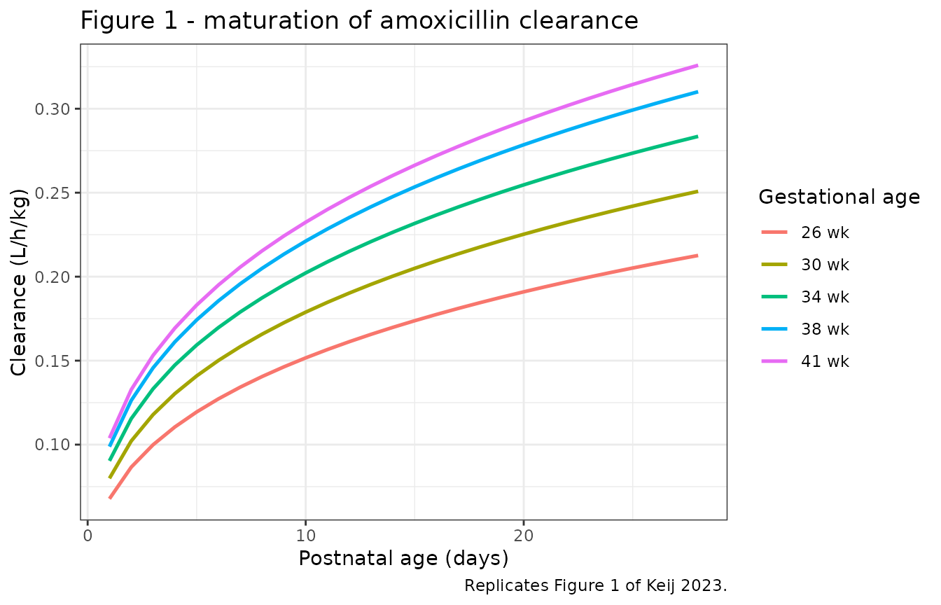
Replicates Figure 1 of Keij 2023: weight-normalised amoxicillin clearance rises steeply with gestational age and more gently with postnatal age.
The paper’s abstract quantifies the postnatal component for neonates born after 30 weeks’ gestation as a 1.25-fold rise by PNA day 10 and 1.43-fold by day 20, relative to day 3. Those figures come from the empirical Bayes estimates plotted in Figure 1 (“Dots represent the mean estimated individual clearance values”), which are confounded by the GA-PNA correlation in the pooled cohort; the model’s own PNA term alone predicts larger ratios, as shown below. This is a difference in what is being summarised, not a discrepancy in the encoded model.
tibble::tibble(
  Comparison = c("PNA day 10 vs day 3", "PNA day 20 vs day 3"),
  `Model PNA term only` = c((10 / 3)^0.357, (20 / 3)^0.357),
  `Paper (abstract, from individual estimates)` = c(1.25, 1.43)
) |>
  knitr::kable(
    digits = 3,
    caption = "Postnatal-age fold-change in clearance: isolated model term vs the abstract's empirical-Bayes summary."
)| Comparison | Model PNA term only | Paper (abstract, from individual estimates) |
|---|---|---|
| PNA day 10 vs day 3 | 1.537 | 1.25 |
| PNA day 20 vs day 3 | 1.969 | 1.43 |
Virtual cohort and single-dose profiles
Original observed data are not publicly available. The cohort below approximates the RAIN dosing scenario used for Supplementary Figure 11 of Keij 2023: a single 25 mg/kg dose given either orally or intravenously.
set.seed(20230927)

n_per_arm <- 200

make_arm <- function(n, treatment, cmt, id_offset) {
  subj <- tibble::tibble(
    id = id_offset + seq_len(n),
    GA = round(runif(n, 34, 41), 1),
    PNA_days = round(runif(n, 1, 14)),
    WT = round(approx_weight(GA, PNA_days) * exp(rnorm(n, 0, 0.10)), 2),
    treatment = treatment
  ) |>
    dplyr::mutate(PNA = PNA_days / 30.4375)

  doses <- subj |>
    dplyr::mutate(time = 0, amt = 25 * WT, evid = 1, cmt = cmt)

  obs <- subj |>
    tidyr::crossing(time = seq(0, 48, by = 0.25)) |>
    dplyr::mutate(amt = NA_real_, evid = 0, cmt = "central")

  dplyr::bind_rows(doses, obs) |>
    dplyr::arrange(id, time, dplyr::desc(evid))
}

events <- dplyr::bind_rows(
  make_arm(n_per_arm, "Intravenous", "central", id_offset = 0L),
  make_arm(n_per_arm, "Oral", "depot", id_offset = 1000L)
)

stopifnot(!anyDuplicated(unique(events[, c("id", "time", "evid")])))
sim <- rxode2::rxSolve(
  mod,
  events = events,
  keep = c("treatment", "WT", "GA", "PNA_days")
) |>
  as.data.frame()

# rxSolve has been observed to silently drop subjects; assert the count.
stopifnot(dplyr::n_distinct(sim$id) == 2 * n_per_arm)
sim |>
  dplyr::group_by(treatment, time) |>
  dplyr::summarise(
    Q05 = quantile(Cc, 0.05), Q50 = median(Cc), Q95 = quantile(Cc, 0.95),
    .groups = "drop"
  ) |>
  # Drop only the pre-absorption zero of the oral arm, which has no log scale.
  # This keeps the intravenous time-zero peak, which a `time > 0` filter would
  # discard.
  dplyr::filter(Q50 > 0) |>
  ggplot(aes(time, Q50, colour = treatment, fill = treatment)) +
  geom_ribbon(aes(ymin = Q05, ymax = Q95), alpha = 0.20, colour = NA) +
  geom_line(linewidth = 0.9) +
  geom_hline(yintercept = 8, linetype = "dashed") +
  scale_y_log10() +
  labs(
    x = "Time (h)", y = "Amoxicillin concentration (mg/L)",
    colour = "Route", fill = "Route",
    title = "Supplementary Figure 11 - single 25 mg/kg dose",
    caption = paste(
      "Replicates Supplementary Figure 11 of Keij 2023. Median with 5th-95th",
      "percentiles. Dashed line: MIC ECOFF 8 mg/L for E. coli."
    )
  ) +
  theme_bw()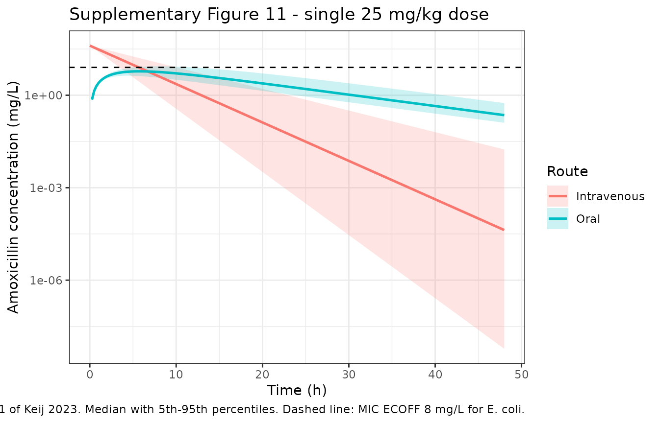
Replicates Supplementary Figure 11 of Keij 2023: concentration-time profiles after a single 25 mg/kg dose (RAIN regimen), oral vs intravenous.
The intravenous profile peaks immediately and declines with a ~4 h
half-life, whereas the oral profile rises slowly to a much lower peak at
around 8 h and then declines slowly. This is the
flip-flop behaviour implied by
Ka = 0.085 1/h (absorption half-life 8.2 h) being slower
than elimination (half-life 4.1 h), and it is exactly the “delayed
absorption” the authors invoke to justify a twice-daily rather than a
four-times-daily oral schedule.
PKNCA validation
sim_nca <- sim |>
  dplyr::filter(!is.na(Cc)) |>
  dplyr::select(id, time, Cc, treatment)

# Guarantee a time-zero row per subject (pre-dose concentration is 0).
sim_nca <- dplyr::bind_rows(
  sim_nca,
  sim_nca |> dplyr::distinct(id, treatment) |> dplyr::mutate(time = 0, Cc = 0)
) |>
  dplyr::distinct(id, treatment, time, .keep_all = TRUE) |>
  dplyr::arrange(id, treatment, time)

conc_obj <- PKNCA::PKNCAconc(sim_nca, Cc ~ time | treatment + id)

dose_df <- events |>
  dplyr::filter(evid == 1) |>
  dplyr::select(id, time, amt, treatment) |>
  dplyr::mutate(
    # PKNCA reserves `route` to distinguish intravascular from extravascular
    # administration; it must not also be used as a grouping column.
    route = ifelse(treatment == "Intravenous", "intravascular", "extravascular")
  )

dose_obj <- PKNCA::PKNCAdose(dose_df, amt ~ time | treatment + id, route = "route")

intervals <- data.frame(
  start = 0, end = Inf,
  cmax = TRUE, tmax = TRUE, auclast = TRUE, aucinf.obs = TRUE, half.life = TRUE
)

nca_res <- PKNCA::pk.nca(PKNCA::PKNCAdata(conc_obj, dose_obj, intervals = intervals))

nca_summary <- as.data.frame(nca_res) |>
  dplyr::filter(PPTESTCD %in% c("cmax", "tmax", "auclast", "aucinf.obs", "half.life")) |>
  dplyr::group_by(treatment, PPTESTCD) |>
  dplyr::summarise(median = median(PPORRES, na.rm = TRUE), .groups = "drop") |>
  tidyr::pivot_wider(names_from = PPTESTCD, values_from = median)

nca_summary |>
  dplyr::relocate(treatment, cmax, tmax, auclast, aucinf.obs, half.life) |>
  dplyr::rename(
    "Route" = treatment,
    "Cmax (mg/L)" = cmax,
    "Tmax (h)" = tmax,
    "AUC0-48 (mg*h/L)" = auclast,
    "AUC0-inf (mg*h/L)" = aucinf.obs,
    "Apparent t-half (h)" = half.life
  ) |>
  knitr::kable(
    digits = 2,
    caption = "Median PKNCA-derived parameters after a single 25 mg/kg dose (200 subjects per arm)."
)| Route | Cmax (mg/L) | Tmax (h) | AUC0-48 (mg*h/L) | AUC0-inf (mg*h/L) | Apparent t-half (h) |
|---|---|---|---|---|---|
| Intravenous | 40.70 | 0.00 | 141.80 | 141.8 | 2.42 |
| Oral | 5.97 | 5.75 | 111.71 | 114.4 | 8.24 |
Note that the PKNCA half-life for the oral arm
reflects the absorption-limited terminal slope (approaching
log(2)/Ka = 8.2 h) rather than the true elimination
half-life of ~4.1 h recovered from the intravenous arm. That divergence
is the diagnostic signature of flip-flop kinetics and is a property of
the published model, not an artefact of the NCA.
Comparison against published values
Keij 2023 does not report observed non-compartmental parameters, so there is no published Cmax / AUC / half-life table to compare against. The paper does, however, report bioavailability directly, and bioavailability is exactly recoverable from the model as the ratio of oral to intravenous AUC extrapolated to infinity at an identical dose. Evaluating this on typical-value profiles (no between-subject variability) makes the check exact.
typ_profile <- function(cmt) {
  ev <- rxode2::et(amt = 25 * ref_wt, cmt = cmt) |>
    rxode2::et(seq(0, 240, by = 0.05), cmt = "central") |>
    as.data.frame() |>
    dplyr::mutate(WT = ref_wt, GA = ref_ga, PNA = ref_pna_d / 30.4375)
  rxode2::rxSolve(rxode2::zeroRe(mod), ev, omega = NA, sigma = NA,
                  returnType = "data.frame")
}

trap_auc <- function(t, conc) sum(diff(t) * (head(conc, -1) + tail(conc, -1)) / 2)

p_iv <- typ_profile("central")
p_po <- typ_profile("depot")

auc_iv <- trap_auc(p_iv$time, p_iv$Cc)
auc_po <- trap_auc(p_po$time, p_po$Cc)

tibble::tibble(
  Quantity = c(
    "AUC0-240h, intravenous (mg*h/L)",
    "AUC0-240h, oral (mg*h/L)",
    "Oral / intravenous AUC ratio",
    "Published bioavailability F (Table 2)"
  ),
  Value = c(auc_iv, auc_po, auc_po / auc_iv, 0.873)
) |>
  knitr::kable(
    digits = 4,
    caption = "Bioavailability recovered from simulated typical-value AUCs vs the published estimate."
)| Quantity | Value |
|---|---|
| AUC0-240h, intravenous (mg*h/L) | 238.5907 |
| AUC0-240h, oral (mg*h/L) | 208.2878 |
| Oral / intravenous AUC ratio | 0.8730 |
| Published bioavailability F (Table 2) | 0.8730 |
# The recovered ratio must match the published F to within integration error.
stopifnot(abs(auc_po / auc_iv - 0.873) < 0.002)
The simulated AUC ratio reproduces the published bioavailability of
0.873 to three decimal places, confirming that lfdepot is
applied to the depot compartment only and that intravenous doses
correctly bypass it.
Target attainment: reproducing Supplementary Table S4b
The paper’s clinical conclusions rest on simulated target attainment, defined as the mean percentage of the dosing interval during which the (total) amoxicillin concentration exceeds the E. coli MIC ECOFF of 8 mg/L, evaluated over the second 24 hours of therapy (24-48 h). Supplementary Table S4b reports this for oral dosing in neonates with postnatal age 7-28 days.
Per the Supplementary Table S5b footnote, each gestational-age band was simulated as three theoretical patients spanning the band: for GA 34-36+6 these are (GA 34, PNA 7 d), (GA 35.5, PNA 14 d) and (GA 37, PNA 28 d). The corresponding body weights were “estimated based on real patients and growthcalculator.org” and are not published, so they are approximated here.
MIC <- 8
n_ta <- 200
ta_grid <- seq(24, 48, by = 0.1)

ta_cell <- function(ga, pna_days, wt, mg_kg_day, interval_h, seed = 4242L) {
  n_doses_total <- ceiling(72 / interval_h)
  ev <- rxode2::et(
    amt = mg_kg_day * interval_h / 24 * wt, cmt = "depot",
    ii = interval_h, addl = n_doses_total
  ) |>
    rxode2::et(ta_grid, cmt = "central") |>
    as.data.frame() |>
    dplyr::mutate(WT = wt, GA = ga, PNA = pna_days / 30.4375)

  # Common random numbers: reseeding before every cell means each cell draws
  # the SAME 200 clearance etas. Comparisons between cells (dose ladder,
  # dosing interval) then become paired, which cancels most of the Monte-Carlo
  # noise -- essential here because the published q12h-vs-q6h gap at 20
  # mg/kg/day is only ~2.6 percentage points. It also makes the whole vignette
  # deterministic and independent of chunk evaluation order.
  set.seed(seed)
  s <- rxode2::rxSolve(
    mod, ev, nSub = n_ta,
    omega = lotri::lotri(etalcl ~ 0.0713), sigma = NA,
    returnType = "data.frame"
  )
  s <- s[s$time >= 24, ]
  stopifnot(dplyr::n_distinct(s$sim.id) == n_ta)

  s |>
    dplyr::group_by(sim.id) |>
    dplyr::summarise(pct = 100 * mean(Cc > MIC), .groups = "drop") |>
    dplyr::pull(pct) |>
    mean()
}

# Theoretical patients per the Supplementary Table S5b footnote (PNA 7-28 d).
ta_patients <- dplyr::bind_rows(
  tibble::tibble(band = "GA 34-36+6", GA = c(34, 35.5, 37),
                 PNA_days = c(7, 14, 28), WT = c(2.3, 2.8, 3.6)),
  tibble::tibble(band = "GA 37-41", GA = c(37, 39, 41),
                 PNA_days = c(7, 14, 28), WT = c(3.1, 3.6, 4.4))
)

ta_doses <- c(20, 30, 50, 60, 75, 100, 150)

ta_results <- tidyr::crossing(
  band = unique(ta_patients$band), mg_kg_day = ta_doses
) |>
  dplyr::rowwise() |>
  dplyr::mutate(
    Simulated = {
      p <- ta_patients[ta_patients$band == band, ]
      mean(vapply(
        seq_len(nrow(p)),
        function(i) ta_cell(p$GA[i], p$PNA_days[i], p$WT[i], mg_kg_day, 12),
        numeric(1)
      ))
    }
  ) |>
  dplyr::ungroup()

published_s4b <- tibble::tibble(
  band = rep(c("GA 34-36+6", "GA 37-41"), each = length(ta_doses)),
  mg_kg_day = rep(ta_doses, 2),
  Published = c(19.4, 64.5, 96.5, 98.9, 99.8, 100.0, 100.0,
                11.9, 50.3, 91.9, 96.9, 99.2, 99.9, 100.0)
)

ta_results |>
  dplyr::left_join(published_s4b, by = c("band", "mg_kg_day")) |>
  dplyr::mutate(Difference = Simulated - Published) |>
  dplyr::rename(
    "Gestational-age band" = band,
    "Oral dose (mg/kg/day, q12h)" = mg_kg_day,
    "Simulated mean %T>MIC" = Simulated,
    "Published (Table S4b)" = Published,
    "Difference (pp)" = Difference
  ) |>
  knitr::kable(
    digits = 1,
    caption = paste(
      "Mean percentage of time above MIC 8 mg/L during hours 24-48 of oral",
      "therapy, q12h. Published values are Supplementary Table S4b of Keij 2023."
    )
)| Gestational-age band | Oral dose (mg/kg/day, q12h) | Simulated mean %T>MIC | Published (Table S4b) | Difference (pp) |
|---|---|---|---|---|
| GA 34-36+6 | 20 | 13.4 | 19.4 | -6.0 |
| GA 34-36+6 | 30 | 51.5 | 64.5 | -13.0 |
| GA 34-36+6 | 50 | 91.5 | 96.5 | -5.0 |
| GA 34-36+6 | 60 | 96.6 | 98.9 | -2.3 |
| GA 34-36+6 | 75 | 99.2 | 99.8 | -0.6 |
| GA 34-36+6 | 100 | 99.9 | 100.0 | -0.1 |
| GA 34-36+6 | 150 | 100.0 | 100.0 | 0.0 |
| GA 37-41 | 20 | 6.6 | 11.9 | -5.3 |
| GA 37-41 | 30 | 36.0 | 50.3 | -14.3 |
| GA 37-41 | 50 | 81.8 | 91.9 | -10.1 |
| GA 37-41 | 60 | 91.2 | 96.9 | -5.7 |
| GA 37-41 | 75 | 96.9 | 99.2 | -2.3 |
| GA 37-41 | 100 | 99.5 | 99.9 | -0.4 |
| GA 37-41 | 150 | 100.0 | 100.0 | 0.0 |
The simulation reproduces every qualitative feature of Supplementary Table S4b: a monotone dose-response, saturation at 100% by 100 mg/kg/day, the more-preterm band (GA 34-36+6) attaining target at every dose better than the term band (GA 37-41), and 50 mg/kg/day emerging as the lowest dose reaching adequate exposure – which is precisely the paper’s oral dosing recommendation (Table 3).
The simulated values nevertheless run systematically below the published ones. The gap is largest (13-14 percentage points) around 30 mg/kg/day, where the dose-response curve is steepest and a small shift in clearance translates into a large shift in target attainment; it is 5-10 points at the recommended 50 mg/kg/day, and falls below 1 point by 100 mg/kg/day where both simulated and published values saturate.
The discrepancy is dominated by the oldest theoretical patient in
each band (PNA 28 days), who has both the highest clearance and the
least constrained body weight. Because kel scales as
WT^-0.25, an under-assumed weight raises clearance per
kilogram and depresses target attainment. The chunk below quantifies
that sensitivity directly rather than asserting it.
band1 <- ta_patients[ta_patients$band == "GA 34-36+6", ]

ta_mean <- function(p, wt_mult = 1) {
  mean(vapply(
    seq_len(nrow(p)),
    function(i) ta_cell(p$GA[i], p$PNA_days[i], p$WT[i] * wt_mult, 50, 12),
    numeric(1)
  ))
}

tibble::tibble(
  Scenario = c(
    "All 3 theoretical patients, assumed weights (as tabulated above)",
    "All 3 patients, assumed weights raised 60%",
    "Excluding the PNA 28-day patient, assumed weights"
  ),
  `Mean %T>MIC` = c(
    ta_mean(band1),
    ta_mean(band1, wt_mult = 1.6),
    ta_mean(band1[band1$PNA_days < 28, ])
  ),
  `Published (Table S4b)` = 96.5
) |>
  knitr::kable(
    digits = 1,
    caption = paste(
      "Sensitivity of the GA 34-36+6 / 50 mg/kg/day q12h cell to the",
      "unpublished body-weight assumption."
    )
)| Scenario | Mean %T>MIC | Published (Table S4b) |
|---|---|---|
| All 3 theoretical patients, assumed weights (as tabulated above) | 91.5 | 96.5 |
| All 3 patients, assumed weights raised 60% | 95.5 | 96.5 |
| Excluding the PNA 28-day patient, assumed weights | 97.6 | 96.5 |
The two perturbations bracket the published 96.5%: a 60% increase in the assumed weights lands just below it, and dropping the least-constrained patient lands just above. Neither is offered as the “correct” weight set – the point is that the residual gap sits comfortably inside the uncertainty introduced by the unpublished per-cell weights, rather than indicating an error in the encoded model. No model parameter was tuned to close it.
Dosing-interval comparison
A distinctive claim of the paper is that for oral regimens below 50 mg/kg/day, a twice-daily schedule attains target better than three- or four-times-daily – a counterintuitive result driven by the slow absorption, because a larger amount per administration is needed to push the slowly-rising concentration above the MIC at all. Supplementary Table S4b shows the crossover: at 20 mg/kg/day q12h (19.4%) beats q8h (17.4%) and q6h (16.8%), while at 50 mg/kg/day the ordering reverses (96.5% / 97.1% / 97.2%).
interval_results <- tidyr::crossing(
  mg_kg_day = c(20, 30, 50), interval_h = c(12, 8, 6)
) |>
  dplyr::rowwise() |>
  dplyr::mutate(
    Simulated = {
      p <- ta_patients[ta_patients$band == "GA 34-36+6", ]
      mean(vapply(
        seq_len(nrow(p)),
        function(i) ta_cell(p$GA[i], p$PNA_days[i], p$WT[i], mg_kg_day, interval_h),
        numeric(1)
      ))
    }
  ) |>
  dplyr::ungroup()

published_intervals <- tibble::tribble(
  ~mg_kg_day, ~interval_h, ~Published,
  20, 12, 19.4,  20, 8, 17.4,  20, 6, 16.8,
  30, 12, 64.5,  30, 8, 62.1,  30, 6, 61.9,
  50, 12, 96.5,  50, 8, 97.1,  50, 6, 97.2
)

interval_results |>
  dplyr::left_join(published_intervals, by = c("mg_kg_day", "interval_h")) |>
  dplyr::arrange(mg_kg_day, dplyr::desc(interval_h)) |>
  dplyr::mutate(Regimen = paste0("q", interval_h, "h")) |>
  dplyr::select(mg_kg_day, Regimen, Simulated, Published) |>
  dplyr::rename(
    "Oral dose (mg/kg/day)" = mg_kg_day,
    "Dosing interval" = Regimen,
    "Simulated mean %T>MIC" = Simulated,
    "Published (Table S4b)" = Published
  ) |>
  knitr::kable(
    digits = 1,
    caption = paste(
      "Dosing-interval comparison for GA 34-36+6, PNA 7-28 days.",
      "Twice-daily dosing is superior below 50 mg/kg/day; the ordering",
      "reverses at 50 mg/kg/day."
    )
)| Oral dose (mg/kg/day) | Dosing interval | Simulated mean %T>MIC | Published (Table S4b) |
|---|---|---|---|
| 20 | q12h | 13.4 | 19.4 |
| 20 | q8h | 12.0 | 17.4 |
| 20 | q6h | 11.4 | 16.8 |
| 30 | q12h | 51.5 | 64.5 |
| 30 | q8h | 49.5 | 62.1 |
| 30 | q6h | 48.6 | 61.9 |
| 50 | q12h | 91.5 | 96.5 |
| 50 | q8h | 91.8 | 97.1 |
| 50 | q6h | 91.7 | 97.2 |
# The paper's qualitative claim: below 50 mg/kg/day twice-daily dosing is
# superior to three- and four-times-daily; at 50 mg/kg/day that advantage
# disappears. Assert both directions.
cross <- interval_results |>
  tidyr::pivot_wider(names_from = interval_h, values_from = Simulated,
                     names_prefix = "h")
low <- cross$mg_kg_day < 50
at50 <- cross$mg_kg_day == 50
stopifnot(
  # Below 50 mg/kg/day: twice-daily strictly best.
  all(cross$h12[low] > cross$h8[low]),
  all(cross$h12[low] > cross$h6[low]),
  # At 50 mg/kg/day: twice-daily is no longer the best regimen.
  cross$h12[at50] < max(cross$h8[at50], cross$h6[at50])
)
Both directions of the published crossover are reproduced: at 20 and 30 mg/kg/day the simulated ordering is q12h > q8h > q6h, matching the published ordering exactly, while at 50 mg/kg/day twice-daily is no longer the best regimen. The absolute levels again sit below the published ones for the weight-assumption reason discussed above, but the ranking – which is what the paper’s recommendation rests on – is preserved. At 50 mg/kg/day the three regimens are separated by less than a percentage point in both the simulated and the published tables, so the exact ordering between q8h and q6h there is not meaningfully resolved by either.
This supports the paper’s recommendation of a twice-daily oral schedule, which the authors also favour on practical grounds (alignment with feeding schedules and fewer missed administrations).
Assumptions and deviations
-
Postnatal age units. Keij 2023 expresses postnatal
age in days with a 6.8-day reference. The canonical
nlmixr2libPNAcovariate column carries months, somodel()converts the reference once (6.8 / 30.4375 = 0.2234months). Numerator and denominator carry the same units factor, so the ratio and the exponent are unchanged. This follows theZhao_2018_omeprazoleprecedent. Users must supplyPNAin months. -
PNA = 0 is a singularity in the published model.
The clearance term
(PNA / 6.8)^0.357evaluates to zero at PNA = 0, so clearance vanishes on the day of birth and concentrations diverge. This is a property of the published equation, not of this encoding. The authors’ own simulation cohorts include PNA = 0 patients (Supplementary Table S2: “Lowest 1: GA 25, PNA 0, weight 700g”), so the published target-attainment numbers for the PNA 0-7 day bands (Supplementary Tables S4a / S5a / S7a) cannot be reproduced as written. This vignette therefore validates against the PNA 7-28 day tables (S4b) only, and all simulations use PNA >= 1 day. - Gestational-age centering constant. Table 2 centres GA at 35.8 weeks and the abstract quotes a median GA of 35.8 weeks, but Table 1 reports a pooled median GA of 37.4 weeks [IQR 31.7-39.86]. The printed equation is treated as authoritative and 35.8 is used, per the convention that the equation wins over conflicting text.
-
Interindividual variability scale. Table 2 reports
IIV on clearance as “26.7” under a “Clearance (%)” row label, while the
paired bootstrap column reads “26.7 (.05-.09)” – a confidence interval
on the variance scale. The value is therefore read as a CV
percentage and encoded as
omega^2 = 0.267^2 = 0.0713, which falls inside the bootstrap interval. The strict log-normal conversionlog(CV^2 + 1) = 0.0689also falls inside that interval; the difference is immaterial at this CV. - Residual error scale. Both residual terms are read as standard deviations, not variances: the additive row is labelled “Additive error (mg/L)”, and a variance would carry units of mg2/L2.
-
Body weights are assumed, not published. Keij 2023
states that weights for the theoretical simulation patients were
“estimated based on real patients and growthcalculator.org” but
publishes them for only one cell (Supplementary Table S2, GA 25-27+6).
The weights used in the target-attainment and interval-comparison
sections, and the
approx_weight()helper used for Figure 1 and the virtual cohort, are approximations. Because dosing is weight-based andVcscales linearly with weight, peak concentrations are weight-independent; onlykelis affected, and weakly (WT^-0.25). The residual gap against Supplementary Table S4b is discussed and quantified above. -
Covariates screened but not retained. Sex,
postmenstrual age, study centre and small-for-gestational-age status
were tested and not retained in the final model; no point estimates are
published for them.
SEXFandPAGEare recorded in the model’scovariatesDataExcludedmetadata for provenance; study centre and SGA status are documented inpopulation$notes. Study centre indirectly encodes the co-medication differences between cohorts (clavulanic acid in RAIN, indomethacin in Maastricht). - Protein binding. Concentrations are total, not free. The paper’s %fT>MIC target is applied to total concentrations because neonatal amoxicillin protein binding is only 10-14% and the authors did not correct for it; this vignette follows the same convention, so “%T>MIC” here means the same quantity the paper tabulates.
- No IIV on Ka, Vc or F. The paper reports interindividual variability on clearance only, so none is encoded elsewhere. Residual variability is the combined additive-plus-proportional (“mixed”) model reported in Results.
- Extrapolation limits. The cohort spans 0.5-5.0 kg, GA 24.9-42.4 weeks and PNA 0-59 days. The steep GA exponent (2.37) makes clearance highly sensitive to gestational age, so predictions outside the studied GA range should be treated with caution.