Islatravir oral and implant PrEP (Kim 2024)
Source:vignettes/articles/Kim_2024_islatravir.Rmd
Kim_2024_islatravir.RmdModel and source
- Citation: Kim S, Zhang L, von Kleist M. Modeling of HIV-1 prophylactic efficacy and toxicity with islatravir shows non-superiority for oral dosing, but promise as a subcutaneous implant. CPT Pharmacometrics Syst Pharmacol. 2024;13(10):1693-1705. doi:10.1002/psp4.13212. PMCID PMC11494919. Structure from Methods Equations (1)-(8) and Figure 1a; PK parameters from Table 1; dose-specific parameters from Supplementary Table S2 and the Figure S6 legend; IC50 from Results; prophylactic-efficacy propensities from Supplementary Text S1 Eqs. (S1)-(S6). Unit conventions and the viral-dynamics constants are from the authors’ code deposit https://github.com/KleistLab/ISL_PK-PD-PrEP (GPL-3.0, commit abc6d6f), whose viral-dynamics model is that of Duwal S, Schuette C, von Kleist M. PLoS One. 2012;7(7):e40382. doi:10.1371/journal.pone.0040382.
- Description: QSP (semi-mechanistic PK-PD with HIV-1 viral dynamics). Islatravir (ISL) for HIV-1 pre-exposure prophylaxis after oral tablets or a subcutaneous (subdermal) implant, from Kim et al. 2024. Plasma ISL is a three-compartment model (central plasma volume fixed at 3.5 L) fed either by first-order oral absorption or by an implant whose first-order release rate decays exponentially from insertion into a subcutaneous compartment that also has its own first-order loss; a loading-dose dependent fraction of the implant load is placed directly in the subcutaneous compartment at insertion. Intracellular ISL-triphosphate (ISL-TP) in peripheral blood mononuclear cells is driven by plasma ISL with a dose- and route-specific uptake/conversion rate and first-order loss. ISL-TP inhibits reverse transcription through an Emax model (IC50 = 429.707 nM) inside an established eight-state HIV-1 viral dynamics model (T cells and macrophages, uninfected / early infected / productively infected, plus infectious and non-infectious virus) that starts at its untreated chronic-infection steady state; the observation is the log10 change from baseline in total plasma virus. Also reports the prophylactic efficacy that the current ISL-TP level would give if held constant. Fitted to published mean concentration-time profiles by least squares: typical-value model with no IIV and no residual error.
- Article: https://doi.org/10.1002/psp4.13212 (open access, PMC11494919)
- Authors’ code and digitised data: https://github.com/KleistLab/ISL_PK-PD-PrEP (GPL-3.0)
- Viral-dynamics source: Duwal S, Schuette C, von Kleist M. PLoS One 2012;7(7):e40382, https://doi.org/10.1371/journal.pone.0040382
Kim et al. built an integrated model of islatravir (ISL) for HIV-1 pre-exposure prophylaxis (PrEP): plasma ISL after an oral tablet or a subcutaneous (subdermal) implant, intracellular ISL-triphosphate (ISL-TP) in peripheral blood mononuclear cells (PBMC), and the effect of ISL-TP on reverse transcription inside an established HIV-1 viral dynamics model. The model was fitted to published mean concentration-time profiles by least squares, so it is a typical-value model: there is no between-subject variability and no residual-error model.
Population
The PK data are mean profiles digitised from five phase 1/2 studies (Supplementary Table S1): ten oral plasma ISL and eleven oral PBMC ISL-TP datasets after single doses of 0.5-400 mg (treatment-naive adults with HIV-1 for 0.5-30 mg; adults without HIV for 5-400 mg), and implant data for loading doses of 48-62 mg in adults without HIV, with the implant removed at week 12 (plasma ISL and ISL-TP at 54 and 62 mg; ISL-TP only at 48, 52 and 56 mg). About 83 of 114 individuals were male, mean age 45.4 years (18-60), mean BMI 26.1 kg/m2 (17.1-32). The antiviral potency IC50 was fitted to mean viral-load declines after single oral doses of 0.5, 1, 2, 10 and 30 mg in 30 treatment-naive men with HIV-1 (6 per dose; Figure 2).
The same information is available programmatically via
readModelDb("Kim_2024_islatravir")()$population.
Source trace
Every ini() value carries an in-file comment naming its
source. The structure is Methods Equations (1)-(8) with Figure 1a.
| Equation / parameter | Value | Source location |
|---|---|---|
d/dt(implant), d/dt(sc)
|
n/a | Eqs. (1)-(2); release clock = time since insertion |
d/dt(depot) |
n/a | Eq. (3) |
d/dt(central) |
n/a | Eq. (4) (equation image) |
d/dt(peripheral1), d/dt(peripheral2)
|
n/a | Eqs. (5)-(6) |
d/dt(pbmc_isltp) |
n/a | Eq. (7) |
eta_rt (Emax inhibition) |
n/a | Eq. (8) |
| viral-dynamics ODEs | n/a | deposit code/steady_state.py,
coupled_ode(); Duwal 2012 |
phi_const |
n/a | Text S1 Eqs. (S1)-(S8); deposit
getExtinctionProbability()
|
lka |
log(0.4232) | Table 1 |
lksc_c, lksc_0
|
log(0.0151), log(0.1521) | Table 1 |
lkel |
log(6.8999) | Table 1, kC->0 |
lk12, lk21
|
log(1.8494), log(0.0023) | Table 1, kC->P1, kP1->C |
lk13, lk31
|
log(5.2726), log(0.0237) | Table 1, kC->P2, kP2->C |
lvc |
fixed log(3.5) | Table 1 / Methods (physiological plasma volume) |
lkel_pbmc |
log(0.0088) | Table 1, kE->0 |
lkr |
log(2.18e-4) | Table S2 |
lkimpl_48 … lkimpl_62
|
log(1.92e-4) … log(4.60e-4) | Table S2 |
lfsc_le54, lfsc_gt54
|
log(0.0412), log(0.0583) | Table S2, pi_ld |
lkce_oral_* (10 doses) |
37.69 … 9.10 | Table S2, kC->E (oral) |
lkce_oral_0p1, _0p25,
_0p75
|
56.64, 40.32, 26.82 | Figure S6 legend |
lkce_implant_* |
25.30 … 36.87 | Table S2, kC->E (implant) |
kce_s6_int, kce_s6_exp
|
4.4, -0.371 | Figure S6 caption |
lic50 |
log(429.707) | Results, “Pharmacodynamics” |
| viral-dynamics constants | see ini()
|
deposit params_vd; Duwal 2012 Table 2 |
Units, and how to dose the model
Doses are in mg. Plasma ISL (Cc, the
central state) is in nM, as in the source. Intracellular
ISL-TP is carried in nM (pbmc_isltp) and reported in pmol
per 10^6 cells as Cpbmc_isltp; the authors’ code converts
between the two with a factor of 5555.6 nM per pmol/10^6 cells (0.18 pL
per PBMC). The viral-load output d_viral_load is the log10
change from baseline in total plasma virus (infectious plus
non-infectious), and phi_const is the prophylactic efficacy
that the current ISL-TP level would give if it were held constant.
Every record carries two covariates: ROUTE_ORAL (1 =
tablet, 0 = implant) and DOSE_ISLATRAVIR_MG (the oral dose
per administration, or the implant load). Together they select the
dose-specific parameters of Supplementary Table S2.
-
Oral: dose
amt = <mg>intodepot. -
Implant insertion: dose the full load
twice at the same time, once into
implantand once intosc. The model’sf()givesimplantthe fraction1 - piandscthe fractionpi(4.12% for loads of 54 mg or less, 5.83% above), reproducing the paper’s initial condition. -
Implant removal: a replacement event
(
evid = 5,amt = 0) onimplant, which stops release as in the source.
mod <- readModelDb("Kim_2024_islatravir")
mod_rx <- rxode2::rxode(mod)

oral_events <- function(dose, tau = 24, n = 1, obs) {
  et(amt = dose, cmt = "depot", ii = if (n > 1) tau else 0, addl = n - 1) |>
    et(obs) |>
    as.data.frame() |>
    mutate(DOSE_ISLATRAVIR_MG = dose, ROUTE_ORAL = 1L)
}

implant_events <- function(load, removal = 2016, obs) {
  et(amt = load, cmt = "implant") |>
    et(amt = load, cmt = "sc") |>
    et(time = removal, amt = 0, evid = 5, cmt = "implant") |>
    et(obs) |>
    as.data.frame() |>
    mutate(DOSE_ISLATRAVIR_MG = load, ROUTE_ORAL = 0L)
}

# Long dosing runs with no intermediate observations exhaust lsoda's default
# step budget, so every solve raises it.
solve_typical <- function(ev) {
  rxode2::rxSolve(mod, events = ev, maxsteps = 1e6, returnType = "data.frame")
}
Virtual cohort
The model has no random effects, so every simulation below is a single typical subject per regimen: there is no cohort to draw. The covariates are regimen descriptors (route and nominal dose), not subject characteristics.
Observed data
The authors deposited their digitised mean profiles with the code. They are embedded here (plasma ISL in nM, ISL-TP in pmol/10^6 cells, time in hours; viral-load change in log10 copies/mL, time in days).
obs_row <- function(type, dose, time, value) {
  tibble(type = type, dose = dose, time = time, obs = value)
}
vl_row <- function(dose, time, change) {
  tibble(dose = dose, time_day = time, obs = change)
}
pk_obs <- dplyr::bind_rows(
  obs_row("implant_intra", 48,
    c(0.7224, 5.477, 9.89, 30.03, 50.2, 99.24, 170.7, 240.2, 335.8, 503.9, 671.8, 1008, 1344, 1680, 2014, 2185, 2349, 2516),
    c(0.01991, 0.06269, 0.1894, 0.2009, 0.3093, 0.338, 0.2575, 0.1595, 0.1713, 0.1764, 0.1513, 0.1531, 0.146, 0.118, 0.1055, 0.05909, 0.01866, 0.01316)
  ),
  obs_row("implant_intra", 52,
    c(0.4, 2.234, 7.806, 44.2, 92.86, 164.2, 237.7, 336.6, 503.3, 670.5, 1004, 1342, 1680, 2013, 2184, 2351, 2518, 2688),
    c(0.03271, 0.0763, 0.199, 0.3479, 0.3281, 0.3583, 0.2951, 0.2849, 0.29, 0.2986, 0.2578, 0.2849, 0.2319, 0.2292, 0.139, 0.04066, 0.02312, 0.01155)
  ),
  obs_row("implant_intra", 54,
    c(1.218, 2.915, 10.9, 20.71, 49.79, 95.96, 166.7, 241.3, 339.1, 503.3, 674.1, 1011, 1344, 1682, 2015, 2352, 2692),
    c(0.03764, 0.09629, 0.2037, 0.2617, 0.2828, 0.24, 0.274, 0.1883, 0.1246, 0.187, 0.1401, 0.0881, 0.1222, 0.1451, 0.1396, 0.03647, 0.0165)
  ),
  obs_row("implant_intra", 56,
    c(1.646, 2.15, 9.358, 22.9, 46.36, 100.3, 168.7, 241, 337.1, 504.2, 674.4, 1009, 1349, 1682, 2020, 2182, 2355, 2522, 2687),
    c(0.02997, 0.08605, 0.2442, 0.3357, 0.6456, 0.4724, 0.598, 0.4697, 0.6232, 0.7095, 0.7481, 0.7179, 0.6848, 0.4752, 0.6418, 0.2083, 0.1102, 0.05798, 0.02776)
  ),
  obs_row("implant_intra", 62,
    c(1.327, 3.024, 6.602, 21.16, 45.32, 92.7, 165, 237, 334.5, 502.4, 670.6, 1005, 1343, 1679, 2015, 2351, 2687),
    c(0.0904, 0.147, 0.4834, 0.5486, 0.4845, 0.6032, 0.6742, 0.7634, 0.6864, 0.6334, 0.5526, 0.6494, 0.6259, 0.3696, 0.2993, 0.1388, 0.03577)
  ),
  obs_row("implant_plasma", 54,
    c(1.928, 3.961, 7.94, 11.99, 23.89, 47.93, 94.33, 164.4, 503.9, 674.4, 1010, 1347),
    c(6.135, 4.76, 2.573, 1.588, 0.9388, 0.6692, 0.4974, 0.4917, 0.5506, 0.6197, 0.4712, 0.4602)
  ),
  obs_row("implant_plasma", 62,
    c(1.795, 3.836, 7.818, 11.93, 24, 48.18, 90.35, 161.2, 233.4, 329.7, 499.8, 668.2, 1007, 1342, 1681, 2015),
    c(10.25, 7.816, 4.22, 2.812, 2.108, 1.538, 1.174, 1.095, 1.029, 1.02, 0.8844, 0.9027, 0.8458, 0.749, 0.659, 0.5783)
  ),
  obs_row("oral_intra", 0.5,
    c(4.25, 12.3, 97.85, 122.9, 146.5, 172.1, 244.9, 343.6, 504.5),
    c(0.2218, 0.2368, 0.2627, 0.1832, 0.2194, 0.1415, 0.06351, 0.0254, 0.007)
  ),
  obs_row("oral_intra", 100,
    c(6.248, 12.27, 24.37, 48.5, 96.27, 168.2, 336.1),
    c(11.29, 10.82, 12, 9.039, 6.864, 5.076, 2.361)
  ),
  obs_row("oral_intra", 10,
    c(4.39, 11.88, 24.58, 97.72, 122.6, 147, 171.4, 244, 344.2, 504.1),
    c(1.86, 3.105, 2.145, 1.114, 1.192, 0.7544, 1.064, 0.9741, 0.3825, 0.1852)
  ),
  obs_row("oral_intra", 15,
    c(6.408, 12.53, 24.38, 48.37, 96.62, 168.2, 336),
    c(2.163, 1.611, 3.261, 2.625, 1.945, 1.22, 0.63)
  ),
  obs_row("oral_intra", 1,
    c(1.821, 12.6, 24.62, 97.42, 122.8, 147, 171.5, 244.3, 343.4, 503.6),
    c(0.4094, 0.3594, 0.2521, 0.2157, 0.1978, 0.1825, 0.1712, 0.0813, 0.07466, 0.02333)
  ),
  obs_row("oral_intra", 200,
    c(6.11, 12.19, 24.35, 48.48, 96.27, 168.1, 336),
    c(36.71, 29.71, 26.28, 21.36, 20.83, 7.713, 4.958)
  ),
  obs_row("oral_intra", 2,
    c(4.24, 12.13, 25.28, 97.73, 122.8, 146.1, 171.6, 244, 343.4, 504),
    c(0.5088, 0.3067, 0.4294, 0.2433, 0.3031, 0.27, 0.2081, 0.1313, 0.0535, 0.0282)
  ),
  obs_row("oral_intra", 30,
    c(3.89, 6.387, 12.25, 12.59, 24.7, 48.1, 96.35, 122.8, 146.9, 171.6, 244.7, 335.9, 343.6, 504.6),
    c(4.912, 6.216, 5.703, 6.124, 6.839, 6.993, 5.172, 3.651, 4.124, 6.06, 1.97, 1.259, 0.7839, 0.1928)
  ),
  obs_row("oral_intra", 400,
    c(6.142, 12.14, 24.21, 96.21, 168.2, 336),
    c(46.9, 52.29, 55.2, 25.75, 18.77, 8.028)
  ),
  obs_row("oral_intra", 5,
    c(6.663, 24.66, 96.36, 168.3, 336.1),
    c(0.589, 0.703, 0.686, 0.393, 0.157)
  ),
  obs_row("oral_plasma", 0.5,
    c(1.9, 3.81, 8.11, 11.98),
    c(6.06, 2.49, 0.76, 0.41)
  ),
  obs_row("oral_plasma", 100,
    c(0.48, 0.99, 1.97, 2.96, 3.92, 5.93, 7.88, 11.93, 15.89, 23.9, 47.99, 96.04),
    c(3143, 2260, 1298, 873.2, 601.8, 293, 164.6, 79.9, 56.53, 43.2, 30.84, 18.76)
  ),
  obs_row("oral_plasma", 10,
    c(0.65, 1.96, 4.03, 7.94, 12.11, 24.08, 48.03, 92.63),
    c(232.3, 133.1, 51.41, 14.53, 7.32, 4.77, 3.38, 2.02)
  ),
  obs_row("oral_plasma", 15,
    c(0.312, 0.942, 2.014, 2.897, 4.032, 5.861, 7.942, 11.92, 15.95, 23.9, 48.18),
    c(328.9, 265.2, 173.7, 112, 73.94, 35.33, 24.05, 12.51, 8.13, 7.136, 5.017)
  ),
  obs_row("oral_plasma", 1,
    c(1.81, 3.8, 8.05, 12.12, 24.2, 48.01),
    c(11.97, 5.04, 1.56, 0.8, 0.41, 0.23)
  ),
  obs_row("oral_plasma", 200,
    c(0.507, 1.016, 2.011, 3.006, 4.005, 6.003, 7.999, 12, 15.89, 23.96, 47.99, 96.1),
    c(6382, 4632, 2993, 1883, 1374, 653.6, 385.8, 170.9, 117.4, 87.69, 63.08, 38.37)
  ),
  obs_row("oral_plasma", 20,
    c(0.212, 1.684, 2.566, 4.038, 5.581, 7.641, 12.21, 24.1, 47.94, 72.01, 96.23),
    c(398.8, 255, 174.2, 113.2, 51.12, 26.8, 12.3, 7.18, 4.706, 3.435, 2.614)
  ),
  obs_row("oral_plasma", 2,
    c(0.33, 0.98, 1.98, 3.82, 8.12, 12.05, 24.07, 48.02, 92.59),
    c(27.64, 28.29, 16.42, 6.5, 1.87, 1.08, 0.75, 0.46, 0.26)
  ),
  obs_row("oral_plasma", 30,
    c(0.25, 0.51, 0.84, 1.02, 2.01, 2.13, 3.01, 4.01, 4.1, 5.99, 8.01, 12.04, 23.98, 48.06, 92.71),
    c(697.8, 1050, 641.2, 731.2, 412.8, 382, 282.8, 197.9, 155, 123.8, 75.1, 22.23, 13.83, 9.88, 5.56)
  ),
  obs_row("oral_plasma", 400,
    c(0.5, 1, 1.99, 2.95, 3.97, 5.97, 7.96, 11.92, 16.01, 23.83, 48.05, 96.06),
    c(9438, 9233, 6231, 4976, 3512, 1824, 1012, 418.8, 261.4, 182.2, 111.5, 64.26)
  ),
  obs_row("oral_plasma", 5,
    c(0.375, 0.879, 1.888, 2.834, 3.843, 5.987, 7.879, 11.92),
    c(150, 106.1, 56.91, 37.85, 28.48, 13.5, 8.315, 4.529)
  )
)
vl_obs <- dplyr::bind_rows(
  vl_row(0.5,
    c(0.1919, 1.034, 4.147, 5.192, 6.237, 7.26),
    c(-0.0331, -0.0881, -0.8834, -1.023, -1.093, -1.21)
  ),
  vl_row(10,
    c(0.1919, 1.045, 4.147, 5.171, 6.205, 7.271, 10.01),
    c(-0.0331, -0.1213, -1.256, -1.591, -1.62, -1.675, -1.788)
  ),
  vl_row(1,
    c(0.2026, 1.034, 4.147, 5.171, 6.247, 7.26),
    c(-0.0884, -0.2319, -0.9019, -1.126, -1.233, -1.299)
  ),
  vl_row(2,
    c(0.2132, 1.045, 4.136, 5.181, 6.237, 7.271),
    c(-0.0626, -0.2061, -0.9719, -1.233, -1.373, -1.347)
  ),
  vl_row(30,
    c(0.1812, 1.034, 4.147, 5.181, 6.237, 7.271, 10.02),
    c(-0.0958, -0.1803, -1.245, -1.473, -1.55, -1.598, -1.877)
  )
)
Viral-dynamics baseline
The viral-dynamics states start at the untreated chronic-infection steady state, which the model computes in closed form. The authors instead ran the untreated system for 200 days from 10^11 uninfected T cells and 10 virions. Both routes must land on the same equilibrium, and the closed-form start must not drift.
ev_none <- et(seq(0, 200 * 24, by = 24)) |>
  as.data.frame() |>
  mutate(DOSE_ISLATRAVIR_MG = 0, ROUTE_ORAL = 1L)
burn_in <- rxode2::rxSolve(
  mod,
  events = ev_none,
  inits = c(
    tcell_uninfected = 2e9 / 0.02, tcell_early = 0, tcell_infected = 0,
    virus = 10, macro_uninfected = 0, macro_early = 0, macro_infected = 0,
    virus_noninfectious = 0
  ),
  returnType = "data.frame"
)
held <- solve_typical(ev_none)

baseline <- tibble(
  State = c("Uninfected T cells", "Productively infected T cells",
            "Infectious virus", "Non-infectious virus"),
  `Closed form` = c(held$tu_ss[1], held$t2_ss[1], held$v_ss[1], held$vn_ss[1]),
  `200-day burn-in` = c(
    tail(burn_in$tcell_uninfected, 1), tail(burn_in$tcell_infected, 1),
    tail(burn_in$virus, 1), tail(burn_in$virus_noninfectious, 1)
  )
)
knitr::kable(baseline, digits = 0, format.args = list(big.mark = ","))| State | Closed form | 200-day burn-in |
|---|---|---|
| Uninfected T cells | 20,403,461,786 | 20,403,461,786 |
| Productively infected T cells | 468,214,931 | 468,214,931 |
| Infectious virus | 13,768,690,889 | 13,768,690,889 |
| Non-infectious virus | 6,878,345,208 | 6,878,345,208 |
Replicate Figure 1: plasma ISL and PBMC ISL-TP
pk_sim <- pk_obs |>
  distinct(type, dose) |>
  rowwise() |>
  do({
    row <- .
    obs_t <- sort(unique(c(seq(0, 3000, by = 2), pk_obs$time[
      pk_obs$type == row$type & pk_obs$dose == row$dose
    ])))
    ev <- if (grepl("oral", row$type)) {
      oral_events(row$dose, obs = obs_t[obs_t <= 700])
    } else {
      implant_events(row$dose, obs = obs_t)
    }
    s <- solve_typical(ev)
    tibble(
      type = row$type, dose = row$dose, time = s$time,
      pred = if (grepl("intra", row$type)) s$Cpbmc_isltp else s$Cc
    )
  }) |>
  ungroup() |>
  distinct(type, dose, time, .keep_all = TRUE)
ggplot(filter(pk_sim, grepl("implant", type), pred > 0), aes(time, pred)) +
  geom_line(aes(colour = factor(dose))) +
  geom_point(
    data = filter(pk_obs, grepl("implant", type)),
    aes(time, obs, colour = factor(dose))
  ) +
  facet_wrap(~type, scales = "free_y", ncol = 1,
             labeller = as_labeller(c(implant_intra = "ISL-TP (pmol/10^6 cells)",
                                      implant_plasma = "Plasma ISL (nM)"))) +
  labs(x = "Time after insertion (h)", y = NULL, colour = "Load (mg)") +
  theme_bw()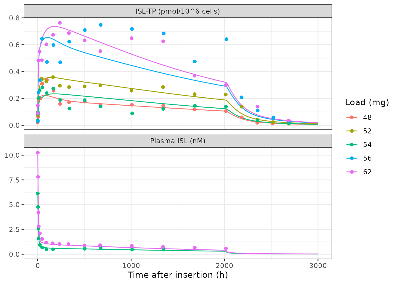
Replicates Figure 1b of Kim 2024: plasma ISL and PBMC ISL-TP after subcutaneous implants (removed at week 12, 2016 h). Points: digitised means from the authors’ deposit; lines: packaged model.
ggplot(filter(pk_sim, grepl("oral", type), pred > 0, time > 0), aes(time, pred)) +
  geom_line(aes(colour = factor(dose))) +
  geom_point(
    data = filter(pk_obs, grepl("oral", type)),
    aes(time, obs, colour = factor(dose))
  ) +
  scale_y_log10() +
  facet_wrap(~type, scales = "free_y", ncol = 1,
             labeller = as_labeller(c(oral_intra = "ISL-TP (pmol/10^6 cells)",
                                      oral_plasma = "Plasma ISL (nM)"))) +
  labs(x = "Time after dose (h)", y = NULL, colour = "Dose (mg)") +
  theme_bw()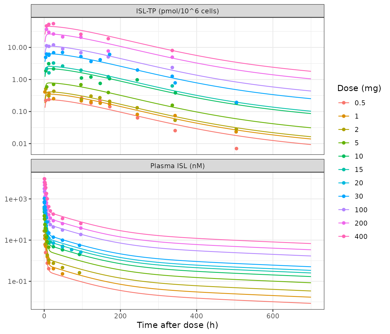
Replicates Figure 1c of Kim 2024: plasma ISL (log scale) and PBMC ISL-TP after single oral doses. Points: digitised means; lines: packaged model.
pk_fit <- pk_obs |>
  inner_join(pk_sim, by = c("type", "dose", "time")) |>
  mutate(log10_err = log10(pred / obs), pct = 100 * (pred - obs) / obs)
stopifnot(nrow(pk_fit) == nrow(pk_obs))

fit_tab <- pk_fit |>
  group_by(type) |>
  summarise(
    n = n(),
    median_abs_pct = median(abs(pct)),
    median_pct = median(pct),
    mean_abs_log10 = mean(abs(log10_err)),
    .groups = "drop"
  )
fit_tab |>
  rename(
    "Data set" = type, "Points" = n,
    "Median |% error|" = median_abs_pct, "Median % error" = median_pct,
    "Mean |log10 error|" = mean_abs_log10
  ) |>
knitr::kable(digits = 2)| Data set | Points | Median |% error| | Median % error | Mean |log10 error| |
|---|---|---|---|---|
| implant_intra | 89 | 18.48 | 0.05 | 0.11 |
| implant_plasma | 28 | 9.31 | -5.76 | 0.06 |
| oral_intra | 85 | 13.02 | -1.22 | 0.08 |
| oral_plasma | 108 | 13.33 | 4.02 | 0.07 |
# A mis-transcribed rate constant or a wrong unit convention for the
# subcutaneous input moves these by tens of percent (the implant plasma set
# is the one that pins the sc unit convention). Measured medians: 9-19%,
# biases within 6%.
stopifnot(
  all(fit_tab$median_abs_pct < 25),
  all(abs(fit_tab$median_pct) < 10)
)
The paper reports average percentage deviations of 11.7% (oral plasma), 2.56% (oral ISL-TP), 12.87% (implant plasma) and 3.8% (implant ISL-TP). The authors fitted the oral data and the ISL-TP data after log10 transformation, and the smaller intracellular figures appear to be computed on that scale; the packaged model’s median absolute errors on the linear scale are in the table above and the agreement is visible in the two figures.
Replicate Figure 2: viral-load decline after a single oral dose
vl_sim <- lapply(unique(vl_obs$dose), function(d) {
  s <- solve_typical(oral_events(d, obs = sort(unique(c(
    seq(0, 11 * 24, by = 2), vl_obs$time_day[vl_obs$dose == d] * 24
  )))))
  tibble(dose = d, time_day = s$time / 24, pred = s$d_viral_load)
}) |>
  bind_rows()

ggplot(vl_sim, aes(time_day, pred)) +
  geom_line() +
  geom_point(data = vl_obs, aes(time_day, obs), colour = "firebrick") +
  geom_hline(yintercept = -1, colour = "grey60") +
  facet_wrap(~dose, labeller = label_both, nrow = 1) +
  labs(x = "Time (days)", y = "log10 change in viral load") +
  theme_bw()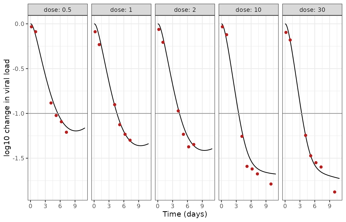
Replicates Figure 2 of Kim 2024: log10 change from baseline in plasma viral load after a single oral dose in treatment-naive adults with HIV-1. Points: digitised means; lines: packaged model.
vl_fit <- vl_obs |>
  mutate(pred = mapply(function(d, t) {
    v <- vl_sim$pred[vl_sim$dose == d & abs(vl_sim$time_day - t) < 1e-9]
    if (length(v) != 1L) stop("no unique prediction for ", d, " mg at day ", t)
    v
  }, dose, time_day))
vl_tab <- vl_fit |>
  group_by(dose) |>
  summarise(mean_abs_diff = mean(abs(pred - obs)), .groups = "drop")
knitr::kable(
  rename(vl_tab, "Dose (mg)" = dose, "Mean |difference| (log10)" = mean_abs_diff),
  digits = 3
)| Dose (mg) | Mean |difference| (log10) |
|---|---|
| 0.5 | 0.050 |
| 1.0 | 0.038 |
| 2.0 | 0.055 |
| 10.0 | 0.081 |
| 30.0 | 0.052 |
Prophylactic efficacy thresholds (Figure S4)
Holding the intracellular ISL-TP concentration constant, the paper
derives the levels giving 85% and 90% reduction in infection risk per
exposure: EC85 = 0.35 and EC90 = 0.51 pmol/10^6 cells.
phi_const reproduces them.
phi_at <- function(pmol) {
  ev <- et(0) |>
    as.data.frame() |>
    mutate(DOSE_ISLATRAVIR_MG = 0, ROUTE_ORAL = 1L)
  rxode2::rxSolve(mod, events = ev, inits = c(pbmc_isltp = pmol * 5555.6),
                  returnType = "data.frame")$phi_const[1]
}
ec <- vapply(c(0.85, 0.90), function(p) {
  uniroot(function(x) phi_at(x) - p, c(0.01, 5), tol = 1e-8)$root
}, numeric(1))
ec_tab <- tibble(
  Threshold = c("EC85", "EC90"),
  `Paper (pmol/10^6 cells)` = c(0.35, 0.51),
  `Model (pmol/10^6 cells)` = ec
)
knitr::kable(ec_tab, digits = 3)| Threshold | Paper (pmol/10^6 cells) | Model (pmol/10^6 cells) |
|---|---|---|
| EC85 | 0.35 | 0.353 |
| EC90 | 0.51 | 0.511 |
Dose-specific uptake for untested oral doses (Figure S6)
For oral doses that were not in the fitted data, the paper reads kC->E off the power law kC->E = x^-0.371 e^4.4, where x is the steady-state plasma maximum of the same dose given once weekly. The model carries the per-mg weekly steady-state maximum (26.62 nM/mg); this check confirms that the packaged plasma model gives that value, and that the power law reproduces the three extrapolated values the paper lists in the Figure S6 legend.
wk <- solve_typical(oral_events(1, tau = 168, n = 60,
                                obs = seq(59 * 168, 60 * 168, by = 0.02)))
cmax_wk_per_mg <- max(wk$Cc)

kce_power <- function(dose) exp(4.4) * (26.62 * dose)^-0.371
s6 <- tibble(
  `Dose (mg)` = c(0.1, 0.25, 0.75),
  `Figure S6 legend` = c(56.64, 40.32, 26.82),
  `Power law` = kce_power(c(0.1, 0.25, 0.75)),
  `Model kce` = vapply(c(0.1, 0.25, 0.75), function(d) {
    solve_typical(oral_events(d, obs = 1))$kce[1]
  }, numeric(1))
)
knitr::kable(s6, digits = 2)| Dose (mg) | Figure S6 legend | Power law | Model kce |
|---|---|---|---|
| 0.10 | 56.64 | 56.64 | 56.64 |
| 0.25 | 40.32 | 40.32 | 40.32 |
| 0.75 | 26.82 | 26.82 | 26.82 |
cat("Weekly steady-state Cmax per mg:", signif(cmax_wk_per_mg, 5), "nM\n")
#> Weekly steady-state Cmax per mg: 26.624 nM

stopifnot(
  abs(cmax_wk_per_mg / 26.62 - 1) < 0.005,
  all(abs(s6$`Power law` / s6$`Figure S6 legend` - 1) < 0.005),
  # an oral dose outside the table takes the power law
  abs(solve_typical(oral_events(3, obs = 1))$kce[1] / kce_power(3) - 1) < 1e-8
)
Replicate Table 2: toxicity threshold and time above it
The paper takes the plasma maximum after 0.25 mg once daily as the no-observed-adverse-effect level (NOAEL, 7.02 nM) and reports, for each regimen at steady state, the fraction of time plasma ISL exceeds it and a plasma AUC expressed per 24 h.
regimen <- function(dose, tau, n) {
  s <- solve_typical(oral_events(dose, tau = tau, n = n,
                                 obs = seq((n - 1) * tau, n * tau, by = 0.02)))
  w <- filter(s, time >= (n - 1) * tau, time < n * tau)
  tibble(
    cmax = max(w$Cc),
    time_above = 100 * mean(w$Cc > 7.02),
    auc_per_24h = sum(diff(s$time) * (head(s$Cc, -1) + tail(s$Cc, -1)) / 2) /
      (tau / 24)
  )
}
# One year of dosing reaches steady state for the slow peripheral I phase
# (kP1->C = 0.0023 1/h, half-life about 300 h).
tab2 <- tribble(
  ~dose, ~regimen, ~tau, ~paper_auc, ~paper_above,
  0.1, "once daily", 24, 12.99, 0.0,
  0.25, "once daily", 24, 32.49, 0.0,
  0.5, "once daily", 24, 64.97, 9.5,
  0.75, "once daily", 24, 97.46, 14.9,
  2, "once weekly", 168, 36.89, 3.4,
  5, "once weekly", 168, 92.21, 5.4,
  10, "once weekly", 168, 184.44, 9.7,
  10, "once biweekly", 336, 92.73, 4.0,
  15, "once biweekly", 336, 139.1, 8.9,
  30, "once monthly", 672, 138.65, 10.8,
  60, "once monthly", 672, 277.29, 19.4
) |>
  rowwise() |>
  mutate(sim = list(regimen(dose, tau, ceiling(365 * 24 / tau)))) |>
  ungroup() |>
  unnest(sim) |>
  mutate(auc_ratio = auc_per_24h / paper_auc)

tab2 |>
  select(dose, regimen, paper_auc, auc_per_24h, auc_ratio, paper_above, time_above) |>
  rename(
    "Dose (mg)" = dose, "Regimen" = regimen,
    "AUC per 24 h, paper (nM h)" = paper_auc,
    "AUC per 24 h, model (nM h)" = auc_per_24h,
    "Model / paper" = auc_ratio,
    "Time above NOAEL, paper (%)" = paper_above,
    "Time above NOAEL, model (%)" = time_above
  ) |>
knitr::kable(digits = 2)| Dose (mg) | Regimen | AUC per 24 h, paper (nM h) | AUC per 24 h, model (nM h) | Model / paper | Time above NOAEL, paper (%) | Time above NOAEL, model (%) |
|---|---|---|---|---|---|---|
| 0.10 | once daily | 12.99 | 14.12 | 1.09 | 0.0 | 0.00 |
| 0.25 | once daily | 32.49 | 35.30 | 1.09 | 0.0 | 1.08 |
| 0.50 | once daily | 64.97 | 70.59 | 1.09 | 9.5 | 9.92 |
| 0.75 | once daily | 97.46 | 105.89 | 1.09 | 14.9 | 15.58 |
| 2.00 | once weekly | 36.89 | 40.34 | 1.09 | 3.4 | 3.37 |
| 5.00 | once weekly | 92.21 | 100.85 | 1.09 | 5.4 | 5.46 |
| 10.00 | once weekly | 184.44 | 201.70 | 1.09 | 9.7 | 12.56 |
| 10.00 | once biweekly | 92.73 | 100.85 | 1.09 | 4.0 | 4.14 |
| 15.00 | once biweekly | 139.10 | 151.27 | 1.09 | 8.9 | 11.21 |
| 30.00 | once monthly | 138.65 | 151.27 | 1.09 | 10.8 | 13.08 |
| 60.00 | once monthly | 277.29 | 302.55 | 1.09 | 19.4 | 24.04 |
noael <- tab2$cmax[tab2$dose == 0.25 & tab2$regimen == "once daily"]
cat("Steady-state Cmax for 0.25 mg once daily:", round(noael, 2),
    "nM (paper NOAEL 7.02 nM)\n")
#> Steady-state Cmax for 0.25 mg once daily: 7.29 nM (paper NOAEL 7.02 nM)

low <- tab2$paper_above < 6
stopifnot(
  abs(noael / 7.02 - 1) < 0.06,
  # Regimens the paper rates safe or near-safe (< 6% of time above the
  # NOAEL): within 1.5 percentage points (measured 0.0-1.1).
  all(abs(tab2$time_above - tab2$paper_above)[low] < 1.5),
  # Higher-exposure regimens: a known deviation, see below. The model sits
  # above the paper by 4-29% relative (measured); the bound still fails if
  # the plasma peak moves by a few tens of percent.
  all((tab2$time_above / tab2$paper_above)[!low] > 1),
  all((tab2$time_above / tab2$paper_above)[!low] < 1.35),
  # The AUC column sits a constant 8% below the model for every oral regimen
  # (measured ratios 1.086-1.092), so the offset is definitional, not a PK
  # discrepancy; a wrong clearance would move the ratio for every row.
  all(abs(tab2$auc_ratio - 1.09) < 0.02)
)
implant_tab <- tribble(
  ~load, ~paper_auc, ~paper_above,
  48, 6.51, 0.0,
  52, 9.2, 0.0,
  54, 10.27, 0.1,
  56, 11.83, 0.2,
  62, 15.71, 0.2
) |>
  rowwise() |>
  mutate(sim = list({
    s <- solve_typical(implant_events(load, obs = seq(0, 2016, by = 0.02))) |>
      filter(time <= 2016) |>
      distinct(time, .keep_all = TRUE)
    tibble(
      auc_per_24h = sum(diff(s$time) * (head(s$Cc, -1) + tail(s$Cc, -1)) / 2) / 84,
      time_above = 100 * mean(s$Cc > 7.02)
    )
  })) |>
  ungroup() |>
  unnest(sim) |>
  mutate(auc_ratio = auc_per_24h / paper_auc)

implant_tab |>
  rename(
    "Load (mg)" = load, "AUC per 24 h, paper (nM h)" = paper_auc,
    "Time above NOAEL, paper (%)" = paper_above,
    "AUC per 24 h, model (nM h)" = auc_per_24h,
    "Time above NOAEL, model (%)" = time_above, "Model / paper" = auc_ratio
  ) |>
knitr::kable(digits = 2)| Load (mg) | AUC per 24 h, paper (nM h) | Time above NOAEL, paper (%) | AUC per 24 h, model (nM h) | Time above NOAEL, model (%) | Model / paper |
|---|---|---|---|---|---|
| 48 | 6.51 | 0.0 | 7.22 | 0.00 | 1.11 |
| 52 | 9.20 | 0.0 | 10.21 | 0.03 | 1.11 |
| 54 | 10.27 | 0.1 | 11.40 | 0.05 | 1.11 |
| 56 | 11.83 | 0.2 | 13.11 | 0.18 | 1.11 |
| 62 | 15.71 | 0.2 | 17.42 | 0.22 | 1.11 |
stopifnot(
  all(abs(implant_tab$time_above - implant_tab$paper_above) < 0.15),
  # Constant ratio across loads again (measured 1.108-1.110).
  max(implant_tab$auc_ratio) - min(implant_tab$auc_ratio) < 0.01
)
The model evaluates every regimen after one year of dosing, when the slow peripheral I phase has reached steady state. The paper does not state the dosing duration it evaluated, and its numbers are not all from one: the 0.25 mg once-daily plasma maximum reaches its NOAEL of 7.02 nM after about one week of dosing in this model and 7.29 nM at full steady state, while its AUC column matches about 25 days. The regimens the paper rates safe or nearly safe are reproduced within about one percentage point of time above the NOAEL. The higher-exposure regimens (10 mg weekly, 15 mg biweekly, 30 and 60 mg monthly) come out 21-29% higher in relative terms (for example 12.6% against 9.7% for 10 mg weekly), which is consistent with the paper evaluating them before steady state. Two of them move up one band of the paper’s colour scale, from 5-10% to 10-15% (10 mg weekly and 15 mg biweekly); the monthly regimens stay in their bands. The AUC column of Table 2 is “plasma AUC for tau = 24 h”; the model’s AUC over one dosing interval, scaled to 24 h, is a constant 9% (oral) or 11% (implant, over the 12-week insertion) above it for every regimen, which points to a different evaluation window or normalisation rather than a different exposure.
Replicate Figure 3: once-daily oral dosing
fig3 <- lapply(c(0.1, 0.25, 0.5), function(d) {
  s <- solve_typical(oral_events(d, tau = 24, n = 30, obs = seq(0, 30 * 24, by = 0.5)))
  tibble(dose = d, time_day = s$time / 24, Cc = s$Cc, Cpbmc = s$Cpbmc_isltp)
}) |>
  bind_rows() |>
  pivot_longer(c(Cc, Cpbmc), names_to = "matrix", values_to = "conc")
thresholds <- tibble(
  matrix = c("Cc", "Cpbmc", "Cpbmc"),
  conc = c(7.02, 0.35, 0.51),
  label = c("NOAEL", "EC85", "EC90")
)
ggplot(fig3, aes(time_day, conc, colour = factor(dose))) +
  geom_line() +
  geom_hline(data = thresholds, aes(yintercept = conc), linetype = "dashed") +
  facet_wrap(~matrix, ncol = 1, scales = "free_y",
             labeller = as_labeller(c(Cc = "Plasma ISL (nM)",
                                      Cpbmc = "ISL-TP (pmol/10^6 cells)"))) +
  labs(x = "Time (days)", y = NULL, colour = "Dose (mg)") +
  theme_bw()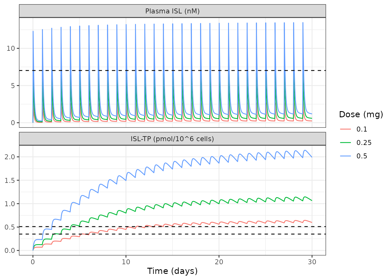
Replicates the once-daily panel of Kim 2024 Figure 3: plasma ISL (top) and PBMC ISL-TP (bottom) for 0.1, 0.25 and 0.5 mg once daily, with the NOAEL and the EC85 / EC90 thresholds.
Implant protection after insertion (Figure 4b, constant-exposure view)
Figure 4b shows the time-resolved prophylactic efficacy, which the
authors compute by solving the extinction-probability equations of Text
S1 backwards in time from each exposure. That backward solve has no
forward-in-time ODE form and is not part of the packaged model.
phi_const, the efficacy the current ISL-TP level would give
if held constant, is shown instead. It is not the same quantity: it
ignores the protection carried forward by ISL-TP that persists after an
exposure, and it drifts down during wear as the release rate decays (for
62 mg from 0.94 in the first week to 0.83 by week 12). It does reproduce
the paper’s ranking of the loads: only 56 and 62 mg ever reach 90%, and
52 mg sits above 54 mg because its fitted ISL-TP uptake is higher (the
paper’s Discussion notes the same inversion in the data).
fig4 <- lapply(c(48, 52, 54, 56, 62), function(ld) {
  s <- solve_typical(implant_events(ld, obs = seq(0, 2400, by = 4)))
  tibble(load = ld, time_day = s$time / 24, phi = s$phi_const)
}) |>
  bind_rows() |>
  distinct(load, time_day, .keep_all = TRUE)
ggplot(fig4, aes(time_day, 100 * phi, colour = factor(load))) +
  geom_line() +
  geom_hline(yintercept = c(85, 90), linetype = c("dashed", "dotted")) +
  geom_vline(xintercept = 84, colour = "red") +
  labs(x = "Time after insertion (days)", y = "Prophylactic efficacy (%)",
       colour = "Load (mg)") +
  theme_bw()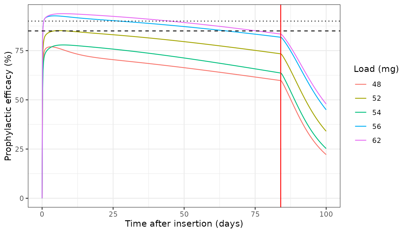
Constant-exposure prophylactic efficacy (phi_const) during 12 weeks of implant wear, by load. Dashed and dotted lines: 85% and 90%.
wear <- fig4 |>
  filter(time_day <= 84) |>
  group_by(load) |>
  summarise(max_phi = max(phi), median_phi = median(phi), .groups = "drop") |>
  arrange(load)
knitr::kable(
  rename(wear, "Load (mg)" = load, "Maximum phi_const" = max_phi,
         "Median phi_const" = median_phi),
  digits = 3
)| Load (mg) | Maximum phi_const | Median phi_const |
|---|---|---|
| 48 | 0.769 | 0.677 |
| 52 | 0.852 | 0.807 |
| 54 | 0.779 | 0.727 |
| 56 | 0.927 | 0.882 |
| 62 | 0.938 | 0.903 |
PKNCA: single oral doses
The paper does not tabulate NCA, but it states that ISL-TP had an intracellular half-life of 87.75 h in the model, in line with the 78.5-128 h reported clinically for 0.5-30 mg. PKNCA on the packaged model’s single-dose profiles gives the apparent terminal half-life of PBMC ISL-TP; the comparison with 87.75 h is discussed under “Assumptions and deviations”.
nca_doses <- c(0.5, 2, 10, 30)
nca_sim <- lapply(nca_doses, function(d) {
  s <- solve_typical(oral_events(d, obs = c(0, 0.25, 0.5, 1, 1.5, 2, 3, 4, 6,
                                            8, 12, 24, 48, 72, 96, 120, 144,
                                            168, 240, 336)))
  tibble(id = 1L, treatment = paste(d, "mg"), dose = d, time = s$time,
         Cc = s$Cc, Cpbmc = s$Cpbmc_isltp)
}) |>
  bind_rows() |>
  distinct(treatment, time, .keep_all = TRUE)

dose_df <- nca_sim |>
  distinct(id, treatment, dose) |>
  mutate(time = 0)

nca_one <- function(col) {
  conc <- nca_sim |>
    rename(conc = all_of(col)) |>
    filter(!is.na(conc))
  o_conc <- PKNCAconc(conc, conc ~ time | treatment + id)
  o_dose <- PKNCAdose(dose_df, dose ~ time | treatment + id)
  intervals <- data.frame(
    start = 0, end = Inf, cmax = TRUE, tmax = TRUE,
    aucinf.obs = TRUE, half.life = TRUE
  )
  as.data.frame(pk.nca(PKNCAdata(o_conc, o_dose, intervals = intervals)))
}
nca_cc <- nca_one("Cc")
nca_pbmc <- nca_one("Cpbmc")

nca_pbmc |>
  filter(PPTESTCD %in% c("cmax", "tmax", "half.life")) |>
  select(treatment, PPTESTCD, PPORRES) |>
  pivot_wider(names_from = PPTESTCD, values_from = PPORRES) |>
  rename("Dose" = treatment, "ISL-TP Cmax (pmol/10^6 cells)" = cmax,
         "Tmax (h)" = tmax, "Terminal t1/2 (h)" = half.life) |>
knitr::kable(digits = 3)| Dose | ISL-TP Cmax (pmol/10^6 cells) | Tmax (h) | Terminal t1/2 (h) |
|---|---|---|---|
| 0.5 mg | 0.234 | 12 | 112.944 |
| 10 mg | 2.164 | 12 | 112.944 |
| 2 mg | 0.411 | 12 | 112.944 |
| 30 mg | 6.303 | 12 | 112.944 |
sim_hl <- nca_pbmc |>
  filter(PPTESTCD == "half.life") |>
  select(treatment, PPTESTCD, PPORRES)
ref_hl <- tibble(treatment = unique(sim_hl$treatment), half.life = 87.75)
cmp <- nlmixr2lib::ncaComparisonTable(
  simulated = sim_hl,
  reference = ref_hl,
  by = "treatment",
  units = c(half.life = "h")
)
knitr::kable(cmp, caption = paste(
  "ISL-TP apparent terminal half-life from PKNCA (0-336 h) against the",
  "87.75 h the paper reports for its model (Discussion). * marks a",
  "difference above 20%."
))| NCA parameter | treatment | Reference | Simulated | % diff |
|---|---|---|---|---|
| t½ (h) | 0.5 mg | 87.8 | 113 | +28.7%* |
| t½ (h) | 10 mg | 87.8 | 113 | +28.7%* |
| t½ (h) | 2 mg | 87.8 | 113 | +28.7%* |
| t½ (h) | 30 mg | 87.8 | 113 | +28.7%* |
# The apparent half-life is longer than the intrinsic log(2)/kE->0 = 78.8 h
# because plasma ISL, fed back from the peripheral I reservoir (Figure S3),
# keeps supplying the PBMC compartment. It must fall inside the 78.5-128 h
# the paper cites from the clinical 0.5-30 mg data (measured 112.9 h), and
# it is dose-independent because the PK is linear in time.
stopifnot(
  all(sim_hl$PPORRES > 78.5 & sim_hl$PPORRES < 128),
  diff(range(sim_hl$PPORRES)) < 0.01
)

# Plasma ISL is linear: dose-normalised Cmax is the same at every dose.
cmax_cc <- nca_cc |>
  filter(PPTESTCD == "cmax") |>
  left_join(distinct(nca_sim, treatment, dose), by = "treatment")
stopifnot(diff(range(cmax_cc$PPORRES / cmax_cc$dose)) /
            mean(cmax_cc$PPORRES / cmax_cc$dose) < 1e-3)
Assumptions and deviations
- Code deposit as a source. The paper prints the structure (Eqs. 1-8, Text S1) and the fitted PK, implant and IC50 values, but not the units of each state, the PBMC unit conversion, or the viral-dynamics constants. These come from the authors’ deposited code (GPL-3.0), which generated the paper’s figures; every value taken from it is marked “deposit” in the model file.
- Viral-dynamics constants differ from Duwal 2012 in three places. The deposit, which produced Figure 2 and the IC50 fit, uses deltaT1 = 0.5/day, deltaT2 = 1.4/day and betaM = 1e-13, whereas Duwal 2012 Table 2 lists deltaT = deltaT1 = 0.02/day, deltaT2 = 1/day and betaM = 1e-14. The deposit values are kept, because IC50 = 429.707 nM was fitted with them; with the Duwal 2012 values the fitted IC50 would not apply.
- Subcutaneous input on the published scale. Eq. 4 adds kSC->C x SC to the plasma concentration without dividing by VC, and the deposit holds SC in nmol. The model keeps that form, so kSC->C and the implant data fit belong together; the implant plasma data are reproduced within 10% (median).
-
Implant clock. Eq. 1 uses time since the start of
the simulation, with the implant always inserted at time 0. The model
uses time since the implant dose (
tad(implant)), which is identical for the paper’s scenarios and also supports a later or repeated insertion. - Implant loads outside the five studied ones return NA for kC->E and the release rate; the paper gives no rule for them (its 48, 52 and 56 mg release rates were interpolated from in vitro release data, not from a formula).
- Untested oral doses use the Figure S6 power law, as the paper did for 0.1, 0.25 and 0.75 mg (whose legend values are also carried as table entries). The paper’s “plasma concentration at steady state” for that law is identified here as the weekly steady-state maximum: it is the only summary for which all three legend values back-solve to the same per-mg concentration (26.62 nM/mg), and the packaged plasma model gives 26.618.
- ISL-TP half-life of 87.75 h. The Discussion gives this as the model’s intracellular half-life, but Table 1’s kE->0 = 0.0088 1/h corresponds to log(2)/0.0088 = 78.8 h. 87.75 h is log(2)/0.0079, and 0.0079 is the starting value of kE->0 in the deposit’s fitting script, so the Discussion figure appears to come from an earlier fit. The model uses the Table 1 estimate. The apparent terminal half-life of the simulated ISL-TP profile (113 h over two weeks) is longer than either, because plasma ISL returning from the slow peripheral compartment keeps feeding the PBMC compartment.
-
Time-resolved prophylactic efficacy (Eq. 9, Figure
4) needs a backward solve of the extinction-probability equations for
each exposure time and is not packaged.
phi_constpackages the constant-exposure efficacy that defines EC85 and EC90. - Clearance of free virus. The viral-load fit uses CL = 23/day (chronic infection) and the prophylactic efficacy uses 2.3/day (at exposure), as in the deposit and Duwal 2012 Table 2.
- No IIV or residual error. The model was fitted to mean profiles by least squares; the paper reports bootstrap standard deviations of the parameters, not between-subject variability.