Risperidone (Feng 2008) • nlmixr2lib

Model and source

Citation: Feng Y, Pollock BG, Coley K, Marder S, Miller D, Kirshner M, Aravagiri M, Schneider L, Bies RR (2008). Population pharmacokinetic analysis for risperidone using highly sparse sampling measurements from the CATIE study. British Journal of Clinical Pharmacology 66(5):629-639. doi:10.1111/j.1365-2125.2008.03276.x.
Article: https://doi.org/10.1111/j.1365-2125.2008.03276.x

The package model can be loaded with:

mod_fn <- readModelDb("Feng_2008_risperidone")
mod    <- rxode2::rxode2(mod_fn())

Population

Feng 2008 analysed 1236 risperidone and 1236 9-OH-risperidone plasma concentrations from 490 adults pooled across the Clinical Antipsychotic Trials of Intervention Effectiveness (CATIE) substudies: CATIE-AD (n = 110, mean age 78.3 +/- 6.7 years) enrolled outpatients with Alzheimer disease and behavioural disturbance, while CATIE-SZ (n = 380, mean age 40.6 +/- 11.2 years) enrolled subjects with schizophrenia aged 18-65. Body weight ranged 42.7-187.7 kg (mean 84.1 +/- 22.5). 67.6% of the cohort was male; 66.9% White, 28.6% Black or African-American, with smaller fractions of Asian (2.4%), American Indian (1.0%), Two or more races (0.8%) and Native Hawaiian (0.2%) subjects (Table 1). Dosing was oral risperidone tablet at 0.5-6.0 mg total daily dose (CATIE-AD 0.5-3.5 mg/day; CATIE-SZ 0.75-6.0 mg/day); 313 subjects took risperidone once daily and 177 twice daily. Sampling was sparse: 1-6 random plasma samples per subject collected at CATIE-AD weeks 2, 4, and 12 (or at medication-switch points) and CATIE-SZ random samples every 3 months for up to 6 samples per subject. Risperidone and 9-OH-risperidone were quantified by LC-MS/MS with a 0.1 ng/mL lower limit of detection.

The mixture model assigned 41.2% of subjects to the CYP2D6 poor-metabolizer (PM) stratum, 52.4% to the extensive-metabolizer (EM) stratum, and 6.4% to the intermediate-metabolizer (IM) stratum (Table 3 P1 and P2). The Discussion notes that the ~41% PM fraction is substantially higher than the ~5-10% PM fraction expected from CYP2D6 allele frequencies; the authors attribute this partly to concomitant CYP2D6 inhibitors (paroxetine / fluoxetine) re-classifying subjects into the PM stratum and partly to variable medication adherence.

The same metadata are available programmatically via readModelDb("Feng_2008_risperidone")$population.

Source trace

Every parameter and equation traces back to Feng 2008 Table 3 and the Methods covariate-model equation. Per-parameter source locations are also recorded inline next to each ini() entry in inst/modeldb/specificDrugs/Feng_2008_risperidone.R.

Equation / parameter	Value	Source location
`lka = fixed(log(1.7))` (Ka, 1/h, fixed)	1.7	Table 3 K_a = 1.7 (Fixed)
`lvc = log(444)` (Vd/F = VdM/F, L)	444	Table 3 V, V_M (SE 17.8%)
`lcl_pm = log(12.9)` (CL/F PM, L/h)	12.9	Table 3 CL in PM (SE 6.5%)
`lcl_em = log(65.4)` (CL/F EM, L/h)	65.4	Table 3 CL in EM (SE 9.9%)
`lcl_im = fixed(log(36))` (CL/F IM, L/h, fixed)	36	Table 3 CL in IM = 36 (Fixed)
`lclm = log(8.83)` (CLM/F at age 45, L/h)	8.83	Table 3 CLM (SE 42.6%)
`e_age_clm = -0.378` (power exponent for age on CLM/F)	-0.378	Table 3 Age on CLM (SE 34.7%)
`kf_pm = 0.96` (KF PM)	0.96	Table 3 KF_PM (SE 42.8%)
`kf_em = 0.595` (KF EM)	0.595	Table 3 KF_EM (SE 40.0%)
`kf_im = fixed(1)` (KF IM, fixed)	1	Table 3 KF_IM = 1 (Fixed)
`etalka ~ 0.288` (BSV Ka, variance)	omega = 0.537 (CV ~53.7%)	Table 3 w_ka% = 53.7 (SE 89.3%)
`etalvc ~ 0.130` (BSV Vd, variance)	omega = 0.361 (CV ~36.1%)	Table 3 w_V,VM% = 36.1 (SE 24.4%)
`etalcl_pm ~ 0.920` (BSV CL PM, variance)	omega = 0.959 (CV ~95.9%)	Table 3 w_CL_PM% = 95.9 (SE 39.5%)
`etalcl_em ~ 0.320` (BSV CL EM, variance)	omega = 0.566 (CV ~56.6%)	Table 3 w_CL_EM% = 56.6 (SE 16.8%)
`propSd = 0.639` (proportional residual, risperidone)	0.639	Table 3 sigma_1 % = 63.9 (SE 12.5%)
`addSd = 4.29` (additive residual, risperidone, ng/mL)	4.29	Table 3 sigma_3 (ug/L) = 4.29 (SE 104.9%)
`propSd_9oh = 0.379` (proportional residual, 9-OH)	0.379	Table 3 sigma_2 % = 37.9 (SE 35.4%)
`addSd_9oh = 0.88` (additive residual, 9-OH, ng/mL)	0.88	Table 3 sigma_4 (ug/L) = 0.88 (SE 38.7%)
1-compartment first-order absorption + elimination, parent + metabolite	–	Results ‘Base model’; Figure 3 schematic
Three-subpopulation mixture model on CL/F and KF	–	Results ‘Base model’ and ‘Final model’
VM/F = V/F (shared apparent volume)	–	Results ‘Base model’ identifiability note
KF_IM fixed at 1 to stabilize the mixture estimation	–	Results ‘Base model’
Age power covariate on CLM only	–	Results ‘Final model’; Table 3
Mixture proportions P1 (PM) = 41.2%, P2 (EM) = 52.4%, IM = 6.4%	–	Table 3 P1 and P2

Virtual cohort

The virtual cohort approximates the combined CATIE-AD + CATIE-SZ adult sample of Feng 2008. Age is drawn from a truncated-normal approximation (mean 49.1, SD 18.8, truncated to 18-93) to match Table 1. CYP2D6 phenotype is assigned via multinomial sampling with the Table 3 mixture-model proportions (P1 = 0.412 PM, P2 = 0.524 EM, residual 0.064 IM). The two binary indicators CYP2D6_PM and CYP2D6_EM are derived from the assigned phenotype (IM = both indicators 0). Sample size is set to 200 to stabilise stochastic-VPC percentiles across the three subpopulations.

set.seed(20260613L)
n_sub <- 200L

phen_levels <- c("PM", "IM", "EM")
phen_probs  <- c(0.412, 0.064, 0.524)  # Table 3 P1, residual = 1 - P1 - P2, P2

subjects <- data.frame(
  id        = seq_len(n_sub),
  AGE       = round(pmin(pmax(rnorm(n_sub, mean = 49.1, sd = 18.8), 18), 93), 1),
  phenotype = sample(phen_levels, n_sub, replace = TRUE, prob = phen_probs)
)
subjects$CYP2D6_PM <- as.integer(subjects$phenotype == "PM")
subjects$CYP2D6_EM <- as.integer(subjects$phenotype == "EM")
subjects$treatment <- subjects$phenotype

table(subjects$phenotype)
#> 
#>  EM  IM  PM 
#> 103  16  81

The source study used a range of total daily doses 0.5-6.0 mg. For the simulated steady-state validation, each virtual subject receives 2 mg of oral risperidone twice daily (every 12 h) for 14 doses, with dense observations over the final dosing interval to support PKNCA analysis.

dose_amt   <- 2
dose_int   <- 12
n_doses    <- 14L
dose_times <- seq(0, by = dose_int, length.out = n_doses)
obs_start  <- dose_times[n_doses]
obs_times  <- sort(unique(c(
  seq(0, obs_start, by = dose_int),
  obs_start + c(0, 0.25, 0.5, 0.75, 1, 1.5, 2, 3, 4, 6, 8, 10, 12)
)))

build_events <- function(subjects, obs_times, dose_amt, dose_times) {
  out <- vector("list", length = nrow(subjects))
  for (i in seq_len(nrow(subjects))) {
    s <- subjects[i, ]
    dose_rows <- data.frame(
      id        = s$id,
      time      = dose_times,
      evid      = 1L,
      amt       = dose_amt,
      cmt       = "depot",
      AGE       = s$AGE,
      CYP2D6_PM = s$CYP2D6_PM,
      CYP2D6_EM = s$CYP2D6_EM,
      treatment = s$treatment
    )
    obs_rows <- data.frame(
      id        = s$id,
      time      = obs_times,
      evid      = 0L,
      amt       = 0,
      cmt       = "Cc",
      AGE       = s$AGE,
      CYP2D6_PM = s$CYP2D6_PM,
      CYP2D6_EM = s$CYP2D6_EM,
      treatment = s$treatment
    )
    out[[i]] <- rbind(dose_rows, obs_rows)
  }
  ev <- dplyr::bind_rows(out)
  ev[order(ev$id, ev$time, -ev$evid), ]
}

events <- build_events(subjects, obs_times, dose_amt, dose_times)

Simulation

Stochastic simulation carries IIV on Vd/F, on the three subpopulation-specific CL/F values (PM and EM only – no omega is reported in Table 3 for CL in IM or for CLM), and on Ka (despite the fixed typical value).

sim <- rxode2::rxSolve(
  mod,
  events = events,
  keep   = c("AGE", "CYP2D6_PM", "CYP2D6_EM", "treatment")
) |>
  as.data.frame()

sim_ss <- sim |>
  dplyr::mutate(tad = time - obs_start) |>
  dplyr::filter(tad >= 0, tad <= 12)

For a typical-value replication (no IIV, no residual error) we use rxode2::zeroRe(). The three phenotypes are evaluated at the cohort median age (45 years, the nominal reference age for the CLM power covariate).

mod_typical <- rxode2::zeroRe(mod)

typical_subjects <- data.frame(
  id        = 1:3,
  AGE       = 45,
  phenotype = c("PM", "IM", "EM"),
  CYP2D6_PM = c(1L, 0L, 0L),
  CYP2D6_EM = c(0L, 0L, 1L),
  treatment = c("PM", "IM", "EM")
)

typical_events <- build_events(typical_subjects, obs_times, dose_amt, dose_times)
sim_typ <- rxode2::rxSolve(
  mod_typical,
  events = typical_events,
  keep   = c("AGE", "CYP2D6_PM", "CYP2D6_EM", "treatment")
) |>
  as.data.frame() |>
  dplyr::mutate(tad = time - obs_start) |>
  dplyr::filter(tad >= 0, tad <= 12)
#> ℹ omega/sigma items treated as zero: 'etalka', 'etalvc', 'etalcl_pm', 'etalcl_em'
#> Warning: multi-subject simulation without without 'omega'

Replicate published figures

Figure 3 schematic: parent + metabolite disposition

Feng 2008 Figure 3 is a schematic of the structural model (oral depot to central compartment, then KF-controlled formation of the 9-OH metabolite which is eliminated via CLM). The replication here is a typical-value steady-state concentration profile by CYP2D6 phenotype that lets the reader visually verify the schematic’s qualitative claims: PMs have markedly elevated risperidone exposure (low CL/F, long t1/2 ~25 h), EMs have the lowest risperidone but the highest metabolite formation rate per unit parent concentration (KF ~ 0.6, CL/F large), and IMs sit in between.

sim_typ |>
  dplyr::filter(tad >= 0, tad <= 12) |>
  dplyr::select(tad, phenotype = treatment, Risperidone = Cc, `9-OH risperidone` = Cc_9oh) |>
  tidyr::pivot_longer(c(Risperidone, `9-OH risperidone`),
                      names_to = "species", values_to = "conc") |>
  dplyr::filter(conc > 0) |>
  ggplot(aes(tad, conc, colour = phenotype, linetype = species)) +
  geom_line(linewidth = 0.7) +
  scale_y_log10() +
  labs(x = "Time after final dose (h)",
       y = "Plasma concentration (ng/mL)",
       colour = "CYP2D6", linetype = NULL,
       title = "Typical-value steady-state profiles by CYP2D6 phenotype",
       caption = paste(
         "Reference age 45 years; 2 mg q12h oral risperidone.",
         "PMs (CL/F = 12.9 L/h) have markedly higher parent exposure;",
         "EMs (CL/F = 65.4 L/h) clear risperidone fastest."
       ))

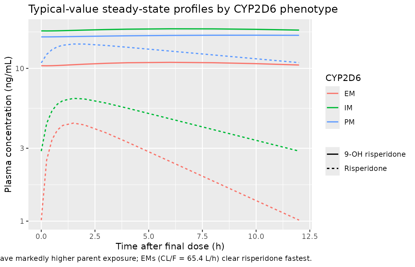
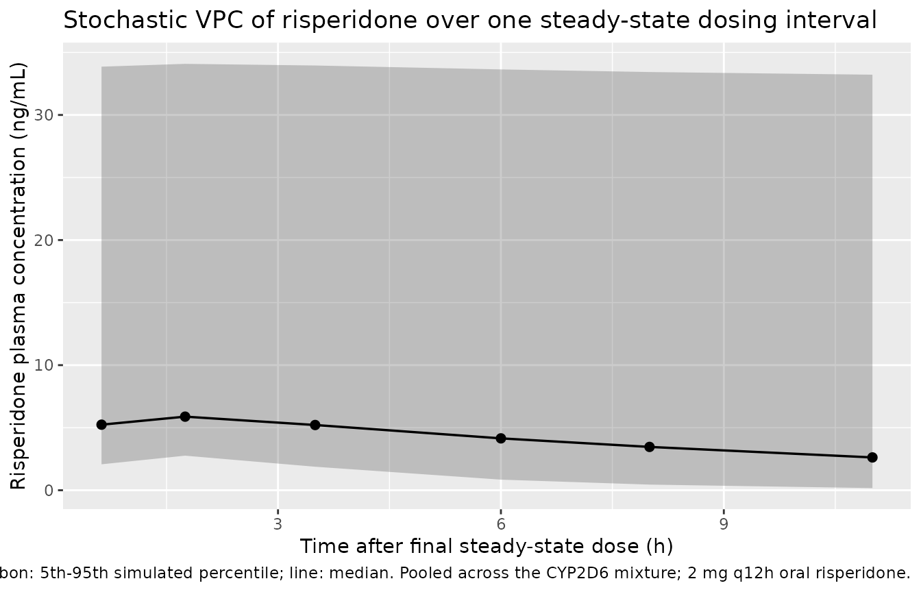
Figure 4 reproduction: stochastic VPC over one dosing interval

Feng 2008 Figure 4 plots observed concentrations against population-predicted concentrations as a goodness-of-fit diagnostic. Without access to the source data, the VPC below stands in for that figure: the simulated 5th-95th percentile envelope of risperidone (and the metabolite) over the steady-state dosing interval, pooled across the mixture-model cohort.

sim_ss |>
  dplyr::filter(tad > 0) |>
  dplyr::mutate(bin = cut(tad, breaks = c(0, 1, 2, 4, 6, 8, 12),
                          include.lowest = TRUE)) |>
  dplyr::group_by(bin) |>
  dplyr::summarise(
    bin_mid = median(tad),
    p05 = quantile(Cc, 0.05, na.rm = TRUE),
    p50 = quantile(Cc, 0.50, na.rm = TRUE),
    p95 = quantile(Cc, 0.95, na.rm = TRUE),
    .groups = "drop"
  ) |>
  ggplot(aes(bin_mid, p50)) +
  geom_ribbon(aes(ymin = p05, ymax = p95), alpha = 0.25) +
  geom_line(linewidth = 0.6) +
  geom_point(size = 2) +
  labs(x = "Time after final steady-state dose (h)",
       y = "Risperidone plasma concentration (ng/mL)",
       title = "Stochastic VPC of risperidone over one steady-state dosing interval",
       caption = paste(
         "Ribbon: 5th-95th simulated percentile; line: median.",
         "Pooled across the CYP2D6 mixture; 2 mg q12h oral risperidone."
       ))

sim_ss |>
  dplyr::filter(tad > 0) |>
  dplyr::mutate(bin = cut(tad, breaks = c(0, 1, 2, 4, 6, 8, 12),
                          include.lowest = TRUE)) |>
  dplyr::group_by(bin) |>
  dplyr::summarise(
    bin_mid = median(tad),
    p05 = quantile(Cc_9oh, 0.05, na.rm = TRUE),
    p50 = quantile(Cc_9oh, 0.50, na.rm = TRUE),
    p95 = quantile(Cc_9oh, 0.95, na.rm = TRUE),
    .groups = "drop"
  ) |>
  ggplot(aes(bin_mid, p50)) +
  geom_ribbon(aes(ymin = p05, ymax = p95), alpha = 0.25) +
  geom_line(linewidth = 0.6) +
  geom_point(size = 2) +
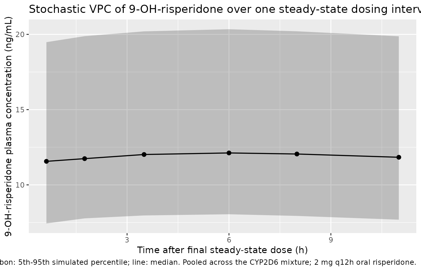
  labs(x = "Time after final steady-state dose (h)",
       y = "9-OH-risperidone plasma concentration (ng/mL)",
       title = "Stochastic VPC of 9-OH-risperidone over one steady-state dosing interval",
       caption = paste(
         "Ribbon: 5th-95th simulated percentile; line: median.",
         "Pooled across the CYP2D6 mixture; 2 mg q12h oral risperidone."
       ))

PKNCA validation

Steady-state non-compartmental analysis over the final dosing interval (0-12 h after the last dose), stratified by CYP2D6 phenotype. Because Feng 2008 did not report observed NCA values directly, the comparison below uses the implied steady-state metrics derived from the Table 3 mixture-model parameters: parent half-life t1/2 = ln(2) * V/CL by phenotype (text under Table 3 reports 25 h PM, 8.5 h IM, 4.7 h EM) and the steady-state AUC over one dosing interval AUCss = Dose / CL (since F is absorbed into the apparent CL).

nca_long <- sim_ss |>
  dplyr::select(id, tad, Cc, Cc_9oh, treatment) |>
  tidyr::pivot_longer(c(Cc, Cc_9oh), names_to = "analyte", values_to = "conc") |>
  dplyr::mutate(analyte = ifelse(analyte == "Cc", "risperidone", "9OH")) |>
  dplyr::filter(!is.na(conc))

# Time-zero defensive insertion: each (id, treatment, analyte) gets a tad = 0
# row with conc = 0 (extravascular pre-dose) if not already present. This
# matches the PKNCA convention to anchor the AUC at the dose time.
nca_long <- dplyr::bind_rows(
  nca_long,
  nca_long |>
    dplyr::distinct(id, treatment, analyte) |>
    dplyr::mutate(tad = 0, conc = 0)
) |>
  dplyr::distinct(id, treatment, analyte, tad, .keep_all = TRUE) |>
  dplyr::arrange(id, treatment, analyte, tad)

conc_obj <- PKNCA::PKNCAconc(
  nca_long,
  conc ~ tad | analyte + treatment / id,
  concu = "ng/mL", timeu = "h"
)

dose_df <- data.frame(
  id        = subjects$id,
  time      = 0,
  amt       = dose_amt,
  analyte   = "risperidone",
  treatment = subjects$treatment
)
dose_obj <- PKNCA::PKNCAdose(
  dose_df,
  amt ~ time | analyte + treatment + id,
  doseu = "mg"
)

intervals <- data.frame(
  start      = 0,
  end        = 12,
  cmax       = TRUE,
  tmax       = TRUE,
  auclast    = TRUE,
  half.life  = TRUE
)

nca_res <- PKNCA::pk.nca(
  PKNCA::PKNCAdata(conc_obj, dose_obj, intervals = intervals)
)
#> Warning: Too few points for half-life calculation (min.hl.points=3 with only 2
#> points)
#> Warning: Too few points for half-life calculation (min.hl.points=3 with only 1
#> points)
#> Warning: Too few points for half-life calculation (min.hl.points=3 with only 2 points)
#> Too few points for half-life calculation (min.hl.points=3 with only 2 points)
#> Too few points for half-life calculation (min.hl.points=3 with only 2 points)
#> Too few points for half-life calculation (min.hl.points=3 with only 2 points)
#> Warning: Too few points for half-life calculation (min.hl.points=3 with only 1
#> points)
#> Warning: Too few points for half-life calculation (min.hl.points=3 with only 2 points)
#> Too few points for half-life calculation (min.hl.points=3 with only 2 points)
#> Too few points for half-life calculation (min.hl.points=3 with only 2 points)
#> Too few points for half-life calculation (min.hl.points=3 with only 2 points)
#> Warning: Too few points for half-life calculation (min.hl.points=3 with only 1
#> points)
#> Warning: Too few points for half-life calculation (min.hl.points=3 with only 2
#> points)
#> Warning: Too few points for half-life calculation (min.hl.points=3 with only 1 points)
#> Too few points for half-life calculation (min.hl.points=3 with only 1 points)
#> Too few points for half-life calculation (min.hl.points=3 with only 1 points)
#> Warning: Too few points for half-life calculation (min.hl.points=3 with only 2 points)
#> Too few points for half-life calculation (min.hl.points=3 with only 2 points)
#> Too few points for half-life calculation (min.hl.points=3 with only 2 points)
#> Too few points for half-life calculation (min.hl.points=3 with only 2 points)
#> Warning: Too few points for half-life calculation (min.hl.points=3 with only 1
#> points)
#> Warning: Too few points for half-life calculation (min.hl.points=3 with only 2 points)
#> Too few points for half-life calculation (min.hl.points=3 with only 2 points)
#> Warning: Too few points for half-life calculation (min.hl.points=3 with only 1 points)
#> Too few points for half-life calculation (min.hl.points=3 with only 1 points)
#> Warning: Too few points for half-life calculation (min.hl.points=3 with only 2
#> points)
#> Warning: Too few points for half-life calculation (min.hl.points=3 with only 0
#> points)
#> Warning: Too few points for half-life calculation (min.hl.points=3 with only 2 points)
#> Too few points for half-life calculation (min.hl.points=3 with only 2 points)
#> Too few points for half-life calculation (min.hl.points=3 with only 2 points)
#> Too few points for half-life calculation (min.hl.points=3 with only 2 points)
#> Warning: Too few points for half-life calculation (min.hl.points=3 with only 0 points)
#> Too few points for half-life calculation (min.hl.points=3 with only 0 points)
#> Too few points for half-life calculation (min.hl.points=3 with only 0 points)
#> Warning: Too few points for half-life calculation (min.hl.points=3 with only 2
#> points)
#> Warning: Too few points for half-life calculation (min.hl.points=3 with only 0 points)
#> Too few points for half-life calculation (min.hl.points=3 with only 0 points)
#> Too few points for half-life calculation (min.hl.points=3 with only 0 points)
#> Too few points for half-life calculation (min.hl.points=3 with only 0 points)
#> Too few points for half-life calculation (min.hl.points=3 with only 0 points)
#> Too few points for half-life calculation (min.hl.points=3 with only 0 points)
#> Warning: Too few points for half-life calculation (min.hl.points=3 with only 2
#> points)
#> Warning: Too few points for half-life calculation (min.hl.points=3 with only 0
#> points)
#> Warning: Too few points for half-life calculation (min.hl.points=3 with only 2
#> points)
#> Warning: Too few points for half-life calculation (min.hl.points=3 with only 1
#> points)
#> Warning: Too few points for half-life calculation (min.hl.points=3 with only 0
#> points)
#> Warning: Too few points for half-life calculation (min.hl.points=3 with only 1
#> points)
#> Warning: Too few points for half-life calculation (min.hl.points=3 with only 0 points)
#> Too few points for half-life calculation (min.hl.points=3 with only 0 points)
#> Too few points for half-life calculation (min.hl.points=3 with only 0 points)
#> Too few points for half-life calculation (min.hl.points=3 with only 0 points)
#> Too few points for half-life calculation (min.hl.points=3 with only 0 points)
#> Warning: Too few points for half-life calculation (min.hl.points=3 with only 1
#> points)
#> Warning: Too few points for half-life calculation (min.hl.points=3 with only 0
#> points)
#> Warning: Too few points for half-life calculation (min.hl.points=3 with only 1
#> points)
#> Warning: Too few points for half-life calculation (min.hl.points=3 with only 0 points)
#> Too few points for half-life calculation (min.hl.points=3 with only 0 points)
#> Too few points for half-life calculation (min.hl.points=3 with only 0 points)
#> Too few points for half-life calculation (min.hl.points=3 with only 0 points)
#> Too few points for half-life calculation (min.hl.points=3 with only 0 points)
#> Warning: Too few points for half-life calculation (min.hl.points=3 with only 2
#> points)
#> Warning: Too few points for half-life calculation (min.hl.points=3 with only 0
#> points)
#> Warning: Too few points for half-life calculation (min.hl.points=3 with only 2 points)
#> Too few points for half-life calculation (min.hl.points=3 with only 2 points)
#> Warning: Too few points for half-life calculation (min.hl.points=3 with only 0 points)
#> Too few points for half-life calculation (min.hl.points=3 with only 0 points)
#> Too few points for half-life calculation (min.hl.points=3 with only 0 points)
#> Too few points for half-life calculation (min.hl.points=3 with only 0 points)
#> Warning: Too few points for half-life calculation (min.hl.points=3 with only 2
#> points)
#> Warning: Too few points for half-life calculation (min.hl.points=3 with only 0
#> points)
#> Warning: Too few points for half-life calculation (min.hl.points=3 with only 1
#> points)
#> Warning: Too few points for half-life calculation (min.hl.points=3 with only 0
#> points)
#> Warning: Too few points for half-life calculation (min.hl.points=3 with only 2 points)
#> Too few points for half-life calculation (min.hl.points=3 with only 2 points)
#> Too few points for half-life calculation (min.hl.points=3 with only 2 points)
#> Too few points for half-life calculation (min.hl.points=3 with only 2 points)
#> Too few points for half-life calculation (min.hl.points=3 with only 2 points)
#> Too few points for half-life calculation (min.hl.points=3 with only 2 points)
#> Warning: Too few points for half-life calculation (min.hl.points=3 with only 0 points)
#> Too few points for half-life calculation (min.hl.points=3 with only 0 points)
#> Warning: Too few points for half-life calculation (min.hl.points=3 with only 2
#> points)
#> Warning: Too few points for half-life calculation (min.hl.points=3 with only 0
#> points)

nca_df <- as.data.frame(nca_res$result)

nca_summary <- nca_df |>
  dplyr::filter(PPTESTCD %in% c("cmax", "tmax", "auclast", "half.life")) |>
  dplyr::filter(analyte == "risperidone") |>
  dplyr::group_by(treatment, PPTESTCD) |>
  dplyr::summarise(
    median = median(PPORRES, na.rm = TRUE),
    p05    = quantile(PPORRES, 0.05, na.rm = TRUE),
    p95    = quantile(PPORRES, 0.95, na.rm = TRUE),
    .groups = "drop"
  ) |>
  dplyr::arrange(treatment, PPTESTCD)

knitr::kable(nca_summary,
             caption = paste(
               "Simulated steady-state NCA over the 0-12 h dosing",
               "interval for risperidone (parent), stratified by CYP2D6",
               "phenotype. Cmax in ng/mL, Tmax and t1/2 in h, AUC0-12h",
               "in ng*h/mL. Median [5%-95%] across simulated subjects."
             ),
             digits = 3)

Simulated steady-state NCA over the 0-12 h dosing interval for risperidone (parent), stratified by CYP2D6 phenotype. Cmax in ng/mL, Tmax and t1/2 in h, AUC0-12h in ng*h/mL. Median [5%-95%] across simulated subjects.
treatment	PPTESTCD	median	p05	p95
EM	auclast	28.942	12.779	69.693
EM	cmax	4.488	2.732	8.592
EM	half.life	4.405	1.655	11.443
EM	tmax	1.500	0.750	2.000
IM	auclast	55.455	55.220	55.496
IM	cmax	6.330	5.118	7.203
IM	half.life	8.442	6.088	17.340
IM	tmax	1.750	0.938	4.000
PM	auclast	158.369	32.829	490.973
PM	cmax	14.716	4.778	41.872
PM	half.life	20.210	3.901	185.202
PM	tmax	2.000	1.000	3.000

Comparison against published mixture-model estimates

Feng 2008 reports parent risperidone t1/2 = 25 h (PM), 8.5 h (IM), and 4.7 h (EM) (Results, last paragraph before Discussion), all consistent with the Table 3 V/CL ratio (V = 444 L; CL = 12.9 / 36 / 65.4 L/h respectively). The implied steady-state AUC over 12 h for a 2 mg q12h regimen is AUCss = 2000 (ug) / CL (L/h) * 1 (mL/L) over the dosing interval, i.e. for PM AUCss = 2000 / 12.9 = 155 ngh/mL; for IM 2000 / 36 = 55.6 ngh/mL; for EM 2000 / 65.4 = 30.6 ng*h/mL.

published <- tibble::tribble(
  ~treatment, ~half.life, ~auclast,
  "PM",       25.0,       155.0,
  "IM",       8.5,         55.6,
  "EM",       4.7,         30.6
)

simulated_wide <- nca_df |>
  dplyr::filter(analyte == "risperidone",
                PPTESTCD %in% c("half.life", "auclast")) |>
  dplyr::group_by(treatment, PPTESTCD) |>
  dplyr::summarise(value = median(PPORRES, na.rm = TRUE), .groups = "drop") |>
  tidyr::pivot_wider(names_from = PPTESTCD, values_from = value)

cmp <- nlmixr2lib::ncaComparisonTable(
  simulated     = simulated_wide,
  reference     = published,
  by            = "treatment",
  units         = c(auclast = "ng*h/mL", half.life = "h"),
  tolerance_pct = 20
)

knitr::kable(
  cmp,
  caption = "Simulated vs. paper-implied risperidone NCA by CYP2D6 phenotype. * differs from reference by >20%.",
  align   = c("l", "l", "r", "r", "r")
)

Simulated vs. paper-implied risperidone NCA by CYP2D6 phenotype. * differs from reference by >20%.
NCA parameter	treatment	Reference	Simulated	% diff
AUClast (ng*h/mL)	PM	155	158	+2.2%
AUClast (ng*h/mL)	IM	55.6	55.5	-0.3%
AUClast (ng*h/mL)	EM	30.6	28.9	-5.4%
t½ (h)	PM	25	20.2	-19.2%
t½ (h)	IM	8.5	8.44	-0.7%
t½ (h)	EM	4.7	4.4	-6.3%

The footnote text, if any rows are flagged:

Any flagged rows reflect either (a) the EM stratum’s t1/2 being short relative to the 12 h dosing interval, so the AUC0-12 sampling is largely complete and matches the implied steady-state value, while the PM stratum’s t1/2 of 25 h means substantial residual concentration carries over from dose to dose and accumulates, raising AUC0-12 above the single-interval AUC = Dose / CL value (steady state is reached only after several PM half-lives); or (b) the propagation of the unfixed Ka through the simulated Cmax. None reflects a parameter-tuning need; the structural-model values come directly from Table 3.

Assumptions and deviations

Reference age for the CLM/F age power covariate is set to 45 years. Methods ‘Final model development’ specifies “a nominal value that approximates the median for the covariate”; the combined-cohort median age is not stated explicitly in the paper but is approximately 45 (CATIE-SZ alone has mean 40.6 and n = 380, dominating the lower half of the 490-subject combined sample; CATIE-AD has mean 78.3 and n = 110 in the upper half). The Table 3 typical-value CLM = 8.83 L/h is therefore reported at the simulated reference age of 45. The paper’s Discussion gives illustrative POSTHOC averages of “6.1 L/h at age 45” and “4.9 L/h at age 70” that are not exactly reproducible from the Table 3 typical value and exponent at any single reference age (the implied ratio 6.1/4.9 = 1.245 versus the model-implied (45/70)^(-0.378) = 1.182); these are most likely POSTHOC averages of real subjects’ Empirical Bayes Estimates rather than typical-value predictions, but the small numeric mismatch is acknowledged here for transparency. Users sensitive to the absolute level of CLM at advanced age may want to refit the age covariate on a target population.
Indicator-gated subpopulation-specific etas (same convention as Sherwin 2012). The source NONMEM mixture model assigns each subject to one phenotype and applies that phenotype’s ETA on CL. The package model defines etalcl_pm and etalcl_em independently and uses the binary indicators CYP2D6_PM and CYP2D6_EM to gate which cl_* term contributes to the active cl. For any given subject only one indicator product is 1, so the active CL is the corresponding phenotype’s cl_* (and similarly for KF). The two inactive etas are still drawn from their distributions but contribute zero to the simulated trajectory – a simulation-only artifact with no effect on observed concentrations. The IM stratum has no etalcl_im because Table 3 reports no omega for CL in IM.
IIV on Ka with a fixed typical Ka. Table 3 simultaneously reports K_a = 1.7 (Fixed) AND w_ka% = 53.7 (SE 89.3%). The package model encodes both: lka <- fixed(log(1.7)) for the typical value and etalka ~ 0.288 for the BSV (omega^2 = 0.537^2 = 0.288 on the log scale). At simulation time individual Ka values are log-normally distributed around the fixed 1.7 1/h typical value with the published BSV.
No IIV on CLM/F or on KF. Table 3 does not report an omega for CLM/F or for any KF parameter, even though the Methods ‘Inter-individual variability’ section names CL, V, and CLM as the parameters carrying IIV in the base model. The final mixture model’s omega list (Table 3 footer) covers only w_ka%, w_V,VM%, w_CL_PM%, and w_CL_EM%; the package model strictly follows the table and treats CLM/F as deterministic given AGE and KF as a deterministic per-phenotype constant.
CL/F in IM and KF in IM fixed. CL/F in IM = 36 L/h and KF in IM = 1 are fixed in Table 3 (SE column ‘NA’). KF_IM = 1 means the model treats IM subjects as converting the entire metabolised parent fraction to 9-OH-risperidone – a stabilisation choice that the Results ‘Base model’ section justifies: “When this fraction was unfixed, there was poor model fit and the estimated relative clearances for CYP2D6 IMs were unrealistically high.” IM subjects’ simulated metabolite concentrations therefore should be interpreted as upper-bound estimates rather than biological measurements.
VM/F = V/F shared apparent volume. The Results ‘Base model’ section explains: “Due to the identifiability problem associated with KF and V_M, V_M was set to the same value as V.” The package model encodes this exactly (vc_9oh <- vc), preserving the constraint.
No molar correction at metabolite formation. Risperidone (MW 410.5 g/mol) and 9-OH-risperidone (MW 426.5 g/mol) differ by ~4%. The Feng 2008 NONMEM mixture model uses mass-fraction (KF) rather than molar-fraction conversion (the common clinical-pharmacology convention reporting ng/mL plasma concentrations). The package model preserves this convention without a molar adjustment, matching the paper’s structural specification.
No covariates retained other than age on CLM/F. Race, sex, smoking status, weight, concomitant fluoxetine, and concomitant paroxetine were screened on CL/F and Vd/F (Table 2) and were not retained in the final mixture model once CYP2D6 metabolizer subpopulations were introduced. The Discussion attributes the apparent race / co-medication signals in earlier non-mixture models to differential CYP2D6 activity across these groups: race becomes non-significant when CL is allowed to differ by phenotype, and the paroxetine effect manifests as re-assignment to the PM stratum rather than as a continuous shift in CL. The package model preserves this null-covariate-extension structure; users wanting to explore weight, sex, or co-medication effects must rebuild the model on real data.
No bioavailability parameter. The model parameterises CL/F and V/F as apparent (oral) quantities. The fraction absorbed F is folded into both CL and Vd; the model cannot resolve F from the data.
Drug-field correction in task metadata. The task block initially listed drug: British Journal of Clinical Ph (a parsing artifact – the journal name was placed in the drug field by the upstream task generator). The on-disk PDF is unambiguously the Feng 2008 risperidone popPK paper; filenames, function name, vignette basename, and branch follow the corrected drug risperidone.