Itraconazole nanocrystal formulation (Jansen 2023)
Source:vignettes/articles/Jansen_2023_itraconazole.Rmd
Jansen_2023_itraconazole.RmdModel and source
- Citation: Jansen AME, Ter Heine R, Donnelly JP, Blijlevens N, Bruggemann RJM. Repurposing antifungals: population pharmacokinetics of itraconazole and hydroxy-itraconazole following administration of a nanocrystal formulation. J Antimicrob Chemother. 2023;78(5):1219-1224. doi:10.1093/jac/dkad072.
- Description: Semi-mechanistic population PK model for intravenous itraconazole nanocrystal formulation (NCF) and its active metabolite hydroxy-itraconazole in allogeneic haematopoietic cell transplant recipients (Jansen 2023). A nanocrystal-bound itraconazole compartment receives the infusion and dissolves by a fixed first-order rate constant into a two-compartment dissolved-itraconazole disposition model; all eliminated itraconazole (fraction metabolised fixed to 1) enters a one-compartment hydroxy-itraconazole model. Observed itraconazole is the sum of nanocrystal-bound and dissolved concentrations. Allometric weight scaling with fixed exponents 0.75 on clearances and 1 on volumes. All amounts and concentrations are molar, as the source data were converted to molar equivalents before fitting.
- Article: https://doi.org/10.1093/jac/dkad072
- Supplement (figures S1-S5 and the final model NONMEM control stream): https://europepmc.org/article/PMC/PMC10154123
Population
Ten adults (median age 47.5 years, range 22.0-59.0; 50% female; median weight 78.3 kg, range 60.0-92.5 kg) received a matched allogeneic bone marrow transplant after conditioning with idarubicin, cyclophosphamide and total body irradiation, and took part in a prospective open-label Phase II study of itraconazole nanocrystal formulation (NCF) for prophylaxis of invasive fungal disease at Radboud University Medical Center, Nijmegen (Jansen 2023, Table 1). Underlying diseases were acute lymphatic leukaemia (30%), acute myeloid leukaemia (20%), chronic myelomonocytic leukaemia (20%), non-Hodgkin lymphoma (20%) and myelofibrosis (10%).
Every subject received itraconazole NCF 200 mg as a 2 h intravenous infusion twice daily for 2 days, then 200 mg once daily until day 14. Full pharmacokinetic curves were drawn on days 7 and 14, with pre- and post-infusion samples until day 6, pre-infusion samples on days 10 and 12, and washout samples on days 16, 17, 18, 19 and 28. This yielded 471 itraconazole and 471 paired hydroxy-itraconazole concentrations, all above the LLOQ. The study was explicitly not powered to identify covariates, so body weight - entered a priori as fixed allometric scaling - is the only covariate in the model.
The same information is available programmatically via
readModelDb("Jansen_2023_itraconazole")()$population.
Model structure
The published model is a semi-mechanistic parent-metabolite model
(Jansen 2023 Figure S2, and the $MODEL / $PK
blocks of the supplementary final model control stream):
- The infusion enters a nanocrystal-bound
itraconazole compartment (
central_np), from which drug dissolves by a first-order rate constantkNfixed at 4.62 /h (a 9 min dissolution half-life in human plasma). - Dissolved itraconazole follows two-compartment
disposition (
central,peripheral1). - The fraction of itraconazole metabolised to hydroxy-itraconazole was
fixed to 1, so the whole of
CL_Pfeeds the one-compartment hydroxy-itraconazole model (central_ohi); there is noK10in the control stream. - The nanocrystal-bound volume
V_Nis set equal to the itraconazole central volumeV_P1(an explicit assumption of the paper, made in the absence of nanocrystal-bound concentration measurements). - The observed itraconazole concentration is the sum
of the nanocrystal-bound and dissolved concentrations
(
$ERROR: IPRED = LOG(C1 + C4)), which is whatCcreturns here.
All concentrations in the source analysis were converted to molar
equivalents before fitting, so that the fixed fm = 1
conversion is mole-for-mole. The packaged model therefore works in
mmol and mmol/L, matching the y-axis
of Jansen 2023 Figure 1. This vignette converts to mg/L for comparison
against the paper’s reported trough concentrations and
therapeutic-drug-monitoring targets.
# Molecular weights are chemical constants, NOT taken from the paper (the paper
# does not print them). Itraconazole C35H38Cl2N8O4 = 705.6 g/mol (PubChem CID
# 55283); hydroxy-itraconazole C35H38Cl2N8O5 = 721.6 g/mol (PubChem CID 108222).
MW_ITZ <- 705.6
MW_OHI <- 721.6

# 200 mg itraconazole per infusion, expressed in the model's molar dose unit.
dose_mmol <- 200 / MW_ITZ
dose_mmol
#> [1] 0.2834467
Source trace
The per-parameter origin is recorded as an in-file comment next to
each ini() entry in
inst/modeldb/specificDrugs/Jansen_2023_itraconazole.R. The
table below collects them in one place for review. “Control stream”
refers to the FINAL MODEL CONTROL STREAM printed at the end
of the supplementary data document.
| Equation / parameter | Value | Source location |
|---|---|---|
lcl (CL_P) |
4.29 L/h | Table 2 (95% CI 3.85-4.80); control stream $THETA
TVCLP |
lvc (V_P1 = V_N) |
14.1 L | Table 2 (95% CI 11.8-17.2); control stream $THETA
TVVP1/TVVN |
lq (Q_P) |
53.0 L/h | Table 2 (95% CI 45.3-63.4); control stream $THETA
TVQP |
lvp (V_P2) |
1660 L | Table 2 (95% CI 1558-1775); control stream $THETA
TVVP2 |
lcl_ohi (CL_M) |
2.86 L/h | Table 2 (95% CI 2.43-3.33); control stream $THETA
TVCLM |
lvc_ohi (V_M) |
43.1 L | Table 2 (95% CI 36.9-50.4); control stream $THETA
TVVM |
lkdiss (kN) |
4.62 /h, fixed | Methods, “Population pharmacokinetic analysis”; control stream
$PK KN = 4.62
|
e_wt_cl |
0.75, fixed | Methods, “a fixed exponent of 3/4 for (intercompartmental)
clearance”; control stream (WT/70)**0.75
|
e_wt_vc |
1.0, fixed | Methods, “and 1 for volumes of distribution”; control stream
(WT/70)**1
|
etalcl |
var 0.0126 | Control stream $OMEGA “IIV CLP”; Table 2 reports 11.3%
= sqrt(exp(0.0126) - 1) |
etalcl_ohi |
var 0.0506 | Control stream $OMEGA “IIV CLM”; Table 2 reports 22.8%
= sqrt(exp(0.0506) - 1) |
expSd |
sqrt(0.214) | Control stream $SIGMA BLOCK(2) first diagonal; Table 2
Error_P 48.8% = sqrt(exp(0.214) - 1) |
expSd_ohi |
sqrt(0.0358) | Control stream $SIGMA BLOCK(2) second diagonal; Table 2
Error_M 19.1% = sqrt(exp(0.0358) - 1) |
d/dt(central_np) |
n/a | Control stream $PK K41 = KN; dose administered into
COMP=(NANO)
|
d/dt(central), d/dt(peripheral1)
|
n/a | Control stream $PK K12 = QP/VP1,
K21 = QP/VP2, K13 = CLP/VP1 (no K10) |
d/dt(central_ohi) |
n/a | Control stream $PK K13 = CLP/VP1,
K30 = CLM/VM; Methods, fm assumed 1 |
Cc = (central + central_np)/vc |
n/a | Control stream $ERROR: C1 = A(1)/VP1,
C4 = A(4)/VN, IPRED = LOG(C1+C4)
|
Cc_ohi = central_ohi/vc_ohi |
n/a | Control stream $ERROR: C3 = A(3)/VM,
IPRED = LOG(C3); $PK S3 = VM
|
Dosing regimens used below
mod <- readModelDb("Jansen_2023_itraconazole")

# Trial protocol: 200 mg NCF over 2 h, q12h x 4 doses (days 1-2), then q24h
# until day 14 (12 further doses, last at t = 312 h).
trial_doses <- rxode2::et(amt = dose_mmol, dur = 2, ii = 12, addl = 3,
                          cmt = "central_np") |>
  rxode2::et(amt = dose_mmol, dur = 2, time = 48, ii = 24, addl = 11,
             cmt = "central_np")

# Observation rows name an ODE state in `cmt` and select the model endpoint
# with `dvid`. rxode2 requires an observation record of a multi-endpoint model
# to resolve to one of the endpoint compartments; `dvid` does that without
# writing an algebraic observable name into `cmt` (which would inject a
# compartment slot and renumber the states). Every algebraic observable
# (`Cc`, `Cc_np`, `Cc_ohi`) is returned as a column regardless of `dvid`.
obs_rows <- function(times) {
  data.frame(time = times, evid = 0L, amt = NA_real_,
             cmt = "central", dvid = 1L)
}

add_obs <- function(doses, times) {
  bind_rows(as.data.frame(doses), obs_rows(times)) |>
    arrange(time)
}
Replicate Figure 1
Figure 1 of Jansen 2023 shows simulated nanocrystal-bound itraconazole (dotted), itraconazole (solid) and hydroxy-itraconazole (dashed) for a typical individual given the study protocol, on a log y-axis in mmol/L over 144 h. The nanocrystal-bound curve spikes and collapses within minutes of each infusion (dissolution half-life 9 min), so it appears as a near-vertical excursion at each dose.
ev_typ <- add_obs(trial_doses, seq(0, 144, by = 0.05)) |>
  mutate(WT = 70)

sim_typ <- rxode2::rxSolve(mod, ev_typ, omega = NA, addDosing = FALSE,
                           returnType = "data.frame")
#> ℹ parameter labels from comments will be replaced by 'label()'

fig1 <- sim_typ |>
  transmute(
    time,
    `Nanocrystal-bound itraconazole` = Cc_np,
    `Itraconazole (dissolved)`       = Cc - Cc_np,
    `Hydroxy-itraconazole`           = Cc_ohi
  ) |>
  pivot_longer(-time, names_to = "Analyte", values_to = "conc") |>
  filter(conc > 0)

ggplot(fig1, aes(time, conc, linetype = Analyte)) +
  geom_line() +
  scale_y_log10(limits = c(1e-4, 1e-2)) +
  scale_x_continuous(breaks = seq(0, 144, by = 24)) +
  scale_linetype_manual(values = c(
    "Nanocrystal-bound itraconazole" = "dotted",
    "Itraconazole (dissolved)"       = "solid",
    "Hydroxy-itraconazole"           = "dashed"
  )) +
  labs(x = "Time (h)", y = "Concentration (mmol/L)", linetype = NULL,
       caption = "Replicates Figure 1 of Jansen 2023.") +
  theme(legend.position = "bottom")
#> Warning: Removed 444 rows containing missing values or values outside the scale range
#> (`geom_line()`).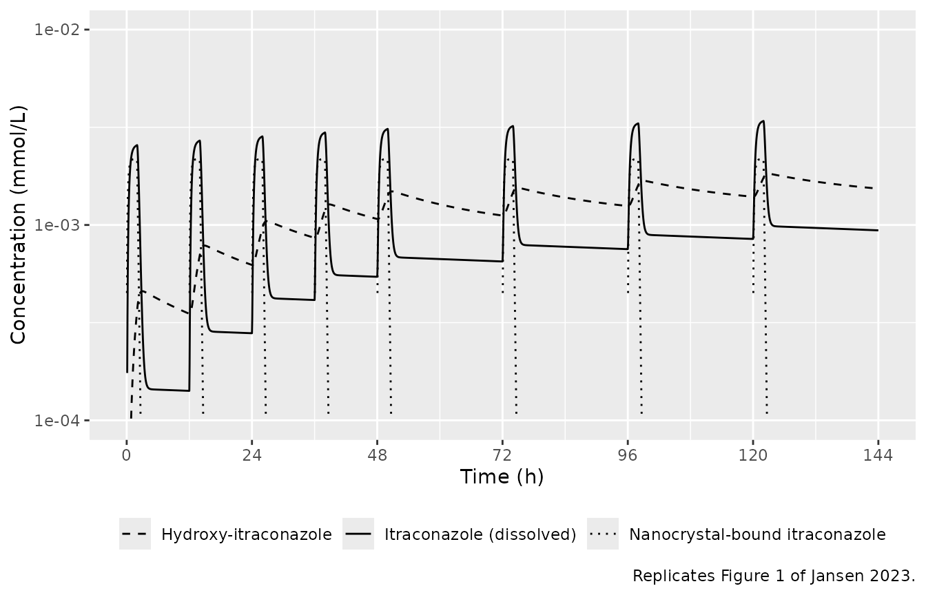
Replicates Figure 1 of Jansen 2023: typical-individual (70 kg) profiles over the first 6 days of the study protocol.
The reproduced curves match the published panel in both level and shape: the itraconazole trough climbs from roughly 1.5e-4 mmol/L after the first inter-dose interval to roughly 9e-4 mmol/L by 144 h, while hydroxy-itraconazole rises smoothly past the parent from about 40 h onward.
tr <- function(t) sim_typ[which.min(abs(sim_typ$time - t)), ]
# Deterministic (typical-value) quantities: a tight bound is appropriate.
stopifnot(
  # Itraconazole trough at 144 h, read off Figure 1 as ~9e-4 mmol/L.
  abs(tr(144)$Cc / 9.0e-4 - 1) < 0.15,
  # Hydroxy-itraconazole overtakes itraconazole partway through the profile
  # and stays above it thereafter, as in Figure 1.
  tr(24)$Cc_ohi  > tr(24)$Cc,
  tr(144)$Cc_ohi > tr(144)$Cc,
  # The nanocrystal-bound term is spent long before the next dose: at the 144 h
  # trough it contributes nothing measurable to the observed itraconazole.
  tr(144)$Cc_np / tr(144)$Cc < 1e-6
)
Virtual cohort
Original observed data are not publicly available. The cohort below reproduces the trial’s body-weight distribution (median 78.3 kg, observed range 60.0-92.5 kg; Jansen 2023 Table 1) and uses the model’s own IIV on itraconazole and hydroxy-itraconazole clearance.
# `set.seed()` seeds R's RNG, not rxode2's, and rxode2's streams are
# partitioned per solver thread -- so this cohort differs between a 2-core CI
# runner and a 16-thread workstation. Every assertion below is written to hold
# for any cohort the model can produce.
set.seed(20230501)

n_sub <- 100  # well under the 200-per-arm cap

cohort <- tibble(
  id = seq_len(n_sub),
  # Log-normal about the published median; SD chosen so the central 95% of the
  # distribution spans roughly the published 60.0-92.5 kg range.
  WT = 78.3 * exp(rnorm(n_sub, 0, 0.12)),
  treatment = "200 mg NCF IV"
)

base_ev <- add_obs(trial_doses, seq(0, 336, by = 0.5))

events <- tidyr::expand_grid(cohort, base_ev) |>
  arrange(id, time)

stopifnot(!anyDuplicated(unique(events[, c("id", "time", "evid")])))Steady-state trough concentrations
Jansen 2023 reports a mean (SD) trough concentration at steady state (after day 7) of 0.79 mg/L (0.35) for itraconazole and 1.31 mg/L (0.29) for hydroxy-itraconazole. Pre-dose samples in that window were drawn on days 7, 10, 12 and 14, i.e. at 144, 216, 264 and 312 h after the first infusion.
The primary comparison uses the typical-value profile at the study’s median weight, which is a deterministic quantity and can therefore be gated tightly.
trough_times <- c(144, 216, 264, 312)

ev_med <- add_obs(trial_doses, trough_times) |>
  mutate(WT = 78.3)

sim_med <- rxode2::rxSolve(mod, ev_med, omega = NA, addDosing = FALSE,
                           returnType = "data.frame")

trough_cmp <- tibble(
  Analyte    = c("Itraconazole", "Hydroxy-itraconazole"),
  Published  = c(0.79, 1.31),
  Simulated  = c(mean(sim_med$Cc) * MW_ITZ, mean(sim_med$Cc_ohi) * MW_OHI)
) |>
  mutate(`% diff` = 100 * (Simulated - Published) / Published)

trough_cmp |>
  rename("Published mean Cmin (mg/L)" = Published,
         "Simulated typical Cmin (mg/L)" = Simulated) |>
  knitr::kable(digits = c(0, 2, 3, 1),
caption = "Mean trough concentration over days 7, 10, 12 and 14 at the study median weight (78.3 kg), against the observed means of Jansen 2023 Results.")| Analyte | Published mean Cmin (mg/L) | Simulated typical Cmin (mg/L) | % diff |
|---|---|---|---|
| Itraconazole | 0.79 | 0.778 | -1.5 |
| Hydroxy-itraconazole | 1.31 | 1.288 | -1.7 |
# Structural gate: a mis-transcribed clearance, dose, molecular weight or unit
# moves these by tens of percent. The typical-value solve is deterministic, so
# the bound does not have to absorb cohort noise.
stopifnot(max(abs(trough_cmp$`% diff`)) < 10)
For context the same window is summarised over the virtual cohort.
Note that these are individual predictions: the published means are
arithmetic means of observations, which the log-scale residual
error would inflate by exp(sigma^2 / 2) (about 11% for
itraconazole and 2% for hydroxy-itraconazole) relative to a noise-free
prediction.
cohort_troughs <- sim |>
  filter(time %in% trough_times) |>
  summarise(
    .by = id,
    ITZ = mean(Cc) * MW_ITZ,
    OHI = mean(Cc_ohi) * MW_OHI
  )

tibble(
  Analyte = c("Itraconazole", "Hydroxy-itraconazole"),
  Median  = c(median(cohort_troughs$ITZ), median(cohort_troughs$OHI)),
  P05     = c(quantile(cohort_troughs$ITZ, 0.05), quantile(cohort_troughs$OHI, 0.05)),
  P95     = c(quantile(cohort_troughs$ITZ, 0.95), quantile(cohort_troughs$OHI, 0.95))
) |>
  rename("Median (mg/L)" = Median, "5th pct" = P05, "95th pct" = P95) |>
  knitr::kable(digits = 3,
caption = "Virtual-cohort mean trough over days 7, 10, 12 and 14 (individual predictions).")| Analyte | Median (mg/L) | 5th pct | 95th pct |
|---|---|---|---|
| Itraconazole | 0.78 | 0.635 | 0.902 |
| Hydroxy-itraconazole | 1.26 | 0.911 | 1.929 |
PKNCA validation
Steady-state exposure over the day-14 dosing interval
PKNCA is used for every NCA quantity. The paper reports
no NCA table, so the values below characterise the packaged model rather
than reproducing a published table.
tau      <- 24
start_ss <- 312          # last dose of the protocol
end_ss   <- start_ss + tau

nca_conc <- function(df, col) {
  out <- df |>
    filter(!is.na(.data[[col]]), time >= start_ss, time <= end_ss) |>
    transmute(id, time, Cc = .data[[col]], treatment)
  out
}

intervals_ss <- data.frame(
  start = start_ss, end = end_ss,
  cmax = TRUE, tmax = TRUE, cmin = TRUE, cav = TRUE, auclast = TRUE
)

dose_df <- events |>
  filter(evid == 1) |>
  transmute(id, time, amt, treatment)

nca_for <- function(col, concu) {
  conc_obj <- PKNCA::PKNCAconc(nca_conc(sim, col), Cc ~ time | treatment + id,
                               concu = concu, timeu = "h")
  dose_obj <- PKNCA::PKNCAdose(dose_df, amt ~ time | treatment + id,
                               doseu = "mmol")
  PKNCA::pk.nca(PKNCA::PKNCAdata(conc_obj, dose_obj, intervals = intervals_ss))
}

nca_itz <- nca_for("Cc", "mmol/L")
nca_ohi <- nca_for("Cc_ohi", "mmol/L")
nca_tbl <- function(res, analyte, mw) {
  as.data.frame(res$result) |>
    filter(PPTESTCD %in% c("cmax", "tmax", "cmin", "cav", "auclast")) |>
    mutate(
      value = if_else(PPTESTCD == "tmax", PPORRES, PPORRES * mw),
      Analyte = analyte
    ) |>
    summarise(.by = c(Analyte, PPTESTCD),
              Median = median(value),
              P05 = quantile(value, 0.05),
              P95 = quantile(value, 0.95)) |>
    mutate(Parameter = nlmixr2lib::ncaParamLabel(PPTESTCD),
           Units = if_else(PPTESTCD == "tmax", "h",
                           if_else(PPTESTCD == "auclast", "mg*h/L", "mg/L"))) |>
    select(Analyte, Parameter, Units, Median, P05, P95)
}

bind_rows(nca_tbl(nca_itz, "Itraconazole", MW_ITZ),
          nca_tbl(nca_ohi, "Hydroxy-itraconazole", MW_OHI)) |>
  rename("5th pct" = P05, "95th pct" = P95) |>
  knitr::kable(digits = 3,
caption = "PKNCA over the day-14 dosing interval (312-336 h) of the virtual cohort, converted from molar to mass units.")| Analyte | Parameter | Units | Median | 5th pct | 95th pct |
|---|---|---|---|---|---|
| Itraconazole | AUClast | mg*h/L | 29.518 | 24.299 | 34.031 |
| Itraconazole | Cmax | mg/L | 3.984 | 3.372 | 4.573 |
| Itraconazole | Cmin | mg/L | 0.922 | 0.746 | 1.064 |
| Itraconazole | Tmax | h | 2.000 | 2.000 | 2.000 |
| Itraconazole | Cavg | mg/L | 1.230 | 1.012 | 1.418 |
| Hydroxy-itraconazole | AUClast | mg*h/L | 39.207 | 28.795 | 58.725 |
| Hydroxy-itraconazole | Cmax | mg/L | 1.764 | 1.312 | 2.579 |
| Hydroxy-itraconazole | Cmin | mg/L | 1.480 | 1.074 | 2.256 |
| Hydroxy-itraconazole | Tmax | h | 3.000 | 3.000 | 3.000 |
| Hydroxy-itraconazole | Cavg | mg/L | 1.634 | 1.200 | 2.447 |
Exact internal identities at true steady state
The terminal half-life implied by the published disposition
parameters is log(2) / beta with beta from the
two-compartment micro-constants; it is long enough (roughly 12 days)
that the 14-day protocol has not reached true steady state, which is why
the troughs above are still climbing at day 14. At true steady state the
model satisfies three exact mass-balance identities, which are checked
here against PKNCA’s AUC over one dosing interval:
-
AUCtau(Cc - Cc_np) = Dose / CL_P- every molecule leaving the dissolved itraconazole compartment does so throughCL_P. -
AUCtau(Cc_np) = Dose / (kN * V_P1)- the nanocrystal-bound compartment has dissolution as its only exit. -
AUCtau(Cc_ohi) = Dose / CL_M-fmis fixed to 1.
n_days <- 120  # about 10 terminal half-lives
t_last <- (n_days - 1) * 24

ev_ss <- add_obs(
  rxode2::et(amt = dose_mmol, dur = 2, ii = 24, addl = n_days - 1,
             cmt = "central_np"),
  seq(t_last, t_last + tau, by = 0.05)
) |>
  mutate(WT = 70, id = 1L, treatment = "200 mg QD to steady state")

sim_ss <- rxode2::rxSolve(mod, ev_ss, omega = NA, addDosing = FALSE,
                          maxsteps = 200000L, atol = 1e-12, rtol = 1e-10,
                          returnType = "data.frame")
if (is.null(sim_ss$id)) sim_ss$id <- 1L
sim_ss$treatment <- "200 mg QD to steady state"

auc_ss <- function(col) {
  conc <- sim_ss |> transmute(id, time, Cc = .data[[col]], treatment)
  conc_obj <- PKNCA::PKNCAconc(conc, Cc ~ time | treatment + id,
                               concu = "mmol/L", timeu = "h")
  dose_obj <- PKNCA::PKNCAdose(
    tibble(id = 1L, time = t_last, amt = dose_mmol,
           treatment = "200 mg QD to steady state"),
    amt ~ time | treatment + id, doseu = "mmol")
  res <- PKNCA::pk.nca(PKNCA::PKNCAdata(
    conc_obj, dose_obj,
    intervals = data.frame(start = t_last, end = t_last + tau, auclast = TRUE)))
  as.data.frame(res$result) |> filter(PPTESTCD == "auclast") |> pull(PPORRES)
}

# The nanocrystal-bound concentration decays through 40 orders of magnitude
# within one dosing interval and its far tail sits in solver round-off, where a
# value can go very slightly negative. PKNCA's log-down trapezoid takes log() of
# it and returns NaN, so clamp the round-off to zero first.
sim_ss$Cc_np   <- pmax(sim_ss$Cc_np, 0)
sim_ss$Cc_free <- sim_ss$Cc - sim_ss$Cc_np
p <- sim_ss[1, ]

identities <- tibble(
  Quantity = c("AUCtau(itraconazole, dissolved)",
               "AUCtau(itraconazole, nanocrystal-bound)",
               "AUCtau(hydroxy-itraconazole)"),
  `Closed form`  = c("Dose / CL_P", "Dose / (kN * V_P1)", "Dose / CL_M"),
  Predicted = c(dose_mmol / p$cl,
                dose_mmol / (p$kdiss * p$vc),
                dose_mmol / p$cl_ohi),
  `PKNCA AUCtau` = c(auc_ss("Cc_free"), auc_ss("Cc_np"), auc_ss("Cc_ohi"))
) |>
  mutate(Ratio = `PKNCA AUCtau` / Predicted)

identities |>
  knitr::kable(digits = c(0, 0, 5, 5, 5),
caption = "Model-internal mass-balance identities at true steady state (200 mg QD, 70 kg, mmol*h/L).")| Quantity | Closed form | Predicted | PKNCA AUCtau | Ratio |
|---|---|---|---|---|
| AUCtau(itraconazole, dissolved) | Dose / CL_P | 0.06607 | 0.06601 | 0.99900 |
| AUCtau(itraconazole, nanocrystal-bound) | Dose / (kN * V_P1) | 0.00435 | 0.00435 | 0.99952 |
| AUCtau(hydroxy-itraconazole) | Dose / CL_M | 0.09911 | 0.09900 | 0.99896 |
# Deterministic: the only error sources are the ODE solver tolerance, the
# trapezoidal AUC rule on a 0.05 h grid, and the residual approach to steady
# state after 120 daily doses. 0.5% is generous for all three together and
# still catches any structural error (a missing elimination path, a wrong
# scaling volume, or an fm that is not 1 move these by tens of percent).
stopifnot(max(abs(identities$Ratio - 1)) < 0.005)
Therapeutic drug monitoring targets
Jansen 2023 simulated day-14 trough concentrations for the standard 200 mg once-daily NCF regimen and compared them against the itraconazole targets of > 0.5 mg/L (prophylaxis) and > 1.0 mg/L (treatment), the itraconazole plus hydroxy-itraconazole targets of > 1.0 mg/L (prophylaxis) and > 2.0 mg/L (treatment), and the itraconazole concentration of > 4.0 mg/L associated with toxicity. The published attainment was 100% / 54.4% for itraconazole, 100% / 91.8% for the sum, and none above the toxicity threshold. This is a partial replication: the published Monte Carlo used the demographics of 1576 haematology patients from the authors’ department, which are not published, so the cohort here uses the trial’s own weight distribution instead.
day14 <- sim |>
  filter(time == 312) |>
  transmute(id,
            ITZ = Cc * MW_ITZ,
            SUM = Cc * MW_ITZ + Cc_ohi * MW_OHI)

targets <- tibble(
  Target = c("Itraconazole Cmin > 0.5 mg/L (prophylaxis)",
             "Itraconazole Cmin > 1.0 mg/L (treatment)",
             "Itraconazole + hydroxy Cmin > 1.0 mg/L (prophylaxis)",
             "Itraconazole + hydroxy Cmin > 2.0 mg/L (treatment)",
             "Itraconazole Cmin > 4.0 mg/L (toxicity)"),
  Published = c(100, 54.4, 100, 91.8, 0),
  Simulated = c(100 * mean(day14$ITZ > 0.5),
                100 * mean(day14$ITZ > 1.0),
                100 * mean(day14$SUM > 1.0),
                100 * mean(day14$SUM > 2.0),
                100 * mean(day14$ITZ > 4.0))
)

targets |>
  rename("Published (%)" = Published, "Simulated (%)" = Simulated) |>
  knitr::kable(digits = 1,
caption = "Day-14 trough target attainment. The published column comes from a Monte Carlo over 1576 haematology patients whose demographics are not reported; the simulated column uses the trial's own weight distribution.")| Target | Published (%) | Simulated (%) |
|---|---|---|
| Itraconazole Cmin > 0.5 mg/L (prophylaxis) | 100.0 | 100 |
| Itraconazole Cmin > 1.0 mg/L (treatment) | 54.4 | 23 |
| Itraconazole + hydroxy Cmin > 1.0 mg/L (prophylaxis) | 100.0 | 100 |
| Itraconazole + hydroxy Cmin > 2.0 mg/L (treatment) | 91.8 | 87 |
| Itraconazole Cmin > 4.0 mg/L (toxicity) | 0.0 | 0 |
# Only the claims the paper states as absolutes are gated, and as proportions
# with headroom rather than as exact 0 / 100. The two treatment-target
# percentages are NOT gated: they depend on a covariate distribution the paper
# does not report.
stopifnot(
  mean(day14$ITZ > 0.5) > 0.95,
  mean(day14$SUM > 1.0) > 0.95,
  mean(day14$ITZ > 4.0) < 0.05
)
The itraconazole treatment target is the one row that does not reproduce, and the reason is visible in the weight sensitivity below. The day-14 trough sits almost exactly on the 1.0 mg/L threshold, so the percentage above it is set by where the simulated population’s weight distribution is centred - the one input this replication cannot reproduce, because the demographics of the paper’s 1576-patient database are not published. A cohort centred near 70 kg puts the typical trough at 1.02 mg/L and therefore roughly half the population above the threshold, which is what the published 54.4% implies; the trial’s own median of 78.3 kg puts it at 0.92 mg/L and only 23% above.
tibble(WT = c(70, 75, 78.3)) |>
  rowwise() |>
  mutate(res = list(rxode2::rxSolve(
    mod, add_obs(trial_doses, 312) |> mutate(WT = WT),
    omega = NA, addDosing = FALSE, returnType = "data.frame"))) |>
  mutate(`Itraconazole (mg/L)` = res$Cc[1] * MW_ITZ,
         `Itraconazole + hydroxy (mg/L)` = res$Cc[1] * MW_ITZ + res$Cc_ohi[1] * MW_OHI) |>
  ungroup() |>
  select(-res) |>
  rename("Body weight (kg)" = WT) |>
  knitr::kable(digits = 3,
caption = "Typical-value day-14 trough as a function of body weight, showing the sensitivity of the 1.0 mg/L treatment target to the simulated population's weight distribution.")| Body weight (kg) | Itraconazole (mg/L) | Itraconazole + hydroxy (mg/L) |
|---|---|---|
| 70.0 | 1.021 | 2.699 |
| 75.0 | 0.959 | 2.537 |
| 78.3 | 0.923 | 2.441 |
Assumptions and deviations
-
Correlated residual error is not reproduced. The
published
$SIGMAis aBLOCK(2)with off-diagonal 0.0185, i.e. a correlation of 0.211 between the itraconazole and hydroxy-itraconazole log-scale residuals. Table 2 reports this as 48.5%, which is the samesqrt(exp(x) - 1)back-transformation the paper applies to its variance terms, evaluated at 0.211 - the two printings are consistent once that is recognised. nlmixr2 has no syntax for a correlated residual-error block across endpoints, so the two residuals are encoded independently. This affects the width of a joint predictive interval for the two analytes, not the typical-value predictions or either marginal residual magnitude. -
Zero-variance IIV terms are omitted. The control
stream declares
$OMEGAentries forV_P1/V_N,Q_P,V_P2andV_Mand fixes all four to0 FIX. Carrying them would make the OMEGA matrix singular and breakrxSolve’s Cholesky sampler, so only the two estimated IIV terms (onCL_PandCL_M) are declared. The model is unchanged. - Molar units, and the molecular weights used here. The packaged model is in mmol and mmol/L because the source data were converted to molar equivalents before fitting (Methods) and Figure 1 is plotted in mmol/L. The molecular weights used in this vignette to convert to mg/L (705.6 g/mol for itraconazole, 721.6 g/mol for hydroxy-itraconazole) are chemical constants from PubChem, not values printed in the paper.
- Body-weight distribution of the virtual cohort, and the one target that does not reproduce. The paper reports only the median (78.3 kg) and range (60.0-92.5 kg) of the trial’s weights, and does not report the demographics of the 1576-patient database used for its own Monte Carlo. The cohort here samples a log-normal with median 78.3 kg and a log-SD of 0.12, which puts the central 95% of the distribution over roughly 62-99 kg. Against that cohort the itraconazole treatment target (Cmin > 1.0 mg/L) is met by about 23% of subjects versus the published 54.4%. This is a known, documented deviation rather than a transcription problem: the day-14 trough is 1.02 mg/L at 70 kg and 0.92 mg/L at 78.3 kg, so the published 54.4% is what a cohort centred near 70 kg would give. Every other published attainment figure reproduces. The two treatment-target rows are deliberately excluded from the vignette’s assertions for this reason.
-
V_N = V_P1is the paper’s own assumption, stated in the Discussion: nanocrystal-bound concentrations were never measured, so the volume of the nanocrystal compartment is not identifiable and was set equal to the itraconazole central volume. -
fm = 1is the paper’s own assumption, made in the absence of metabolic conversion data. Every hydroxy-itraconazole parameter is therefore apparent to the fraction metabolised. - The published trough summary is compared against individual predictions. The paper’s mean Cmin values are arithmetic means of observed concentrations and so include residual error; the typical-value comparison above is noise-free. The log-scale residual would inflate a simulated arithmetic mean by about 11% (itraconazole) and 2% (hydroxy-itraconazole).
- No erratum or corrigendum was found for this article at the time of extraction.