Linezolid + fosfomycin against Enterococcus in vitro (Mao 2021)
Source:vignettes/articles/Mao_2021_linezolid_fosfomycin.Rmd
Mao_2021_linezolid_fosfomycin.RmdModel and source
- Citation: Mao J, Li T, Zhang N, Wang S, Li Y, Peng Y, Liu H, Yang G, Yan Y, Jiang L, Liu Y, Li J, Huang X. Dose optimization of combined linezolid and fosfomycin against Enterococcus by using an in vitro pharmacokinetic/pharmacodynamic model. Microbiol Spectr. 2021;9(3):e00871-21. doi:10.1128/spectrum.00871-21. PMCID: PMC8635129. Structural model: Materials and Methods, ‘Semimechanical PK/PD model’, Equations 1-5. Pharmacodynamic estimates: Table 3, column ATCC 29212. Fosfomycin pharmacokinetics: supplemental Table S1. Interaction (Equation 5) encoded in the form of the cited source, Mohamed AF et al. J Antimicrob Chemother 2016;71(5):1279-1290 (reference 17 of the paper), because the form printed in the paper is inconsistent with its own monotherapy fits
- Article: https://doi.org/10.1128/spectrum.00871-21 (open access, PMC8635129)
- Supplement (Table S1, Figures S1-S4): available from the article landing page.
Mao et al. fit one semimechanistic PK/PD model to dynamic in vitro time-kill data for each of four Enterococcus strains. The model has the same structure for every strain and a strain-specific parameter set (Table 3), so the package ships four files:
strains <- tibble::tribble(
  ~strain,      ~model,                                      ~organism,
  "ATCC 29212", "Mao_2021_linezolid_fosfomycin_ATCC29212",   "E. faecalis (reference strain)",
  "No. 1",      "Mao_2021_linezolid_fosfomycin_strain1",     "E. faecalis",
  "No. 2",      "Mao_2021_linezolid_fosfomycin_strain2",     "linezolid-resistant E. faecium",
  "No. 6",      "Mao_2021_linezolid_fosfomycin_strain6",     "fosfomycin-resistant E. faecium"
)
knitr::kable(strains)| strain | model | organism |
|---|---|---|
| ATCC 29212 | Mao_2021_linezolid_fosfomycin_ATCC29212 | E. faecalis (reference strain) |
| No. 1 | Mao_2021_linezolid_fosfomycin_strain1 | E. faecalis |
| No. 2 | Mao_2021_linezolid_fosfomycin_strain2 | linezolid-resistant E. faecium |
| No. 6 | Mao_2021_linezolid_fosfomycin_strain6 | fosfomycin-resistant E. faecium |
Read this before using the combination model. The monotherapy arms of the packaged models reproduce the published fitted curves. The combination arms, which carry the paper’s headline conclusions, do not reproduce the published Figure 5-7 curves with the printed parameters under any reading of the paper’s interaction equation (Equation 5). The size of the gap is measured below and asserted, so it cannot silently change. Treat combination simulations from these files as a faithful encoding of the printed estimates, not as a reproduction of the authors’ fitted model.
Population
This is an in vitro study (no human or animal subjects). Eight non-duplicate clinical Enterococcus isolates from urine and blood (First Affiliated Hospital of Anhui Medical University) and the CLSI quality-control strain ATCC 29212 were screened by MIC and checkerboard assays (Table 1). The semimechanistic model was fit to the dynamic one-compartment in vitro PK/PD experiments on four strains:
| Strain | Organism | Linezolid MIC (mg/L) | Fosfomycin MIC (mg/L) | Dynamic-model regimens |
|---|---|---|---|---|
| ATCC 29212 | E. faecalis | 2 | 128 | LZD 4, 8 mg/L; FOF 4, 8 g; LZD 4 + FOF 4 g; LZD 8 + FOF 6 g |
| No. 1 | E. faecalis | 4 | 64 | LZD 4, 8 mg/L; FOF 4, 6 g; LZD 4 + FOF 4 g; LZD 8 + FOF 6 g |
| No. 2 | E. faecium, linezolid-resistant | 8 | 128 | LZD 8, 12 mg/L; FOF 6, 8 g; LZD 8 + FOF 6 g; LZD 12 + FOF 8 g |
| No. 6 | E. faecium, fosfomycin-resistant | 2 | 256 | LZD 8, 12 mg/L; FOF 6, 8 g; LZD 8 + FOF 6 g; LZD 12 + FOF 8 g |
Linezolid was held at a constant concentration (added to every
reservoir and the central chamber before the start). Fosfomycin was
given as a simulated human 0.5-h infusion every 8 h following the
two-compartment profile of supplemental Table S1. The starting inoculum
was ~10^6 CFU/mL, viable counts were taken at 0, 2, 4, 6, 8, 10, 12 and
24 h, and the limit of detection was 100 CFU/mL (2 log10 CFU/mL). The
same information is available programmatically,
e.g. readModelDb("Mao_2021_linezolid_fosfomycin_strain2")()$population.
Model structure
With B the viable count on the log10 CFU/mL scale (the paper reports the stationary-phase maximum Bmax in log10 CFU/mL):
- Equations 1-2:
dB/dt = [Kg * (1 - B / Bmax) - E] * B - Equation 3, per drug:
E_drug = Emax * C^Hill / ((alpha * EC50)^Hill + C^Hill) - Equation 4, adaptive resistance:
alpha = 1 + f * (1 - exp(-C * k * t)), with C the current concentration of that drug and t the time since the start of the experiment - Equation 5, combination, encoded as
E = E_LZD * (1 + E_FOF / (E_LZD + E_FOF))^int + E_FOF * (1 + E_LZD / (E_LZD + E_FOF))^int
The paper prints Equation 5 with the same drug’s effect in
each bracket
(E_LZD * [1 + E_LZD / (E_LZD + E_FOF)]^int + ...). That
form multiplies a monotherapy effect by 2^int, which the
paper’s own monotherapy fits rule out (see the check below). The
packaged models therefore use the form of the source the paper cites for
Equation 5 (Mohamed et al. 2016, reference 17; the same form is in
Mohamed_2016_colistin_meropenem), in which each bracket
carries the other drug and the expression reduces to the single drug’s
effect in monotherapy.
Source trace
Every ini() value carries an in-file comment naming its
source. The table collects them.
pars <- c(
  "lkgrow", "log10cfumax", "lemax_lzd", "lec50_lzd", "hill_lzd", "lfadapt_lzd",
  "lkadapt_lzd", "lemax_fof", "lec50_fof", "hill_fof", "lfadapt_fof",
  "lkadapt_fof", "inter"
)
paper_names <- c(
  "Kg (1/h)", "Bmax (log10 CFU/mL)", "Emax-LZD (1/h)", "EC50-LZD (mg/L)",
  "Hill LZD", "f LZD", "k LZD", "Emax-FOF (1/h)", "EC50-FOF (mg/L)",
  "Hill FOF", "f FOF", "k FOF", "Int"
)
theta_of <- function(model_name) {
  th <- rxode2::rxode(readModelDb(model_name))$theta
  out <- th[pars]
  logp <- startsWith(pars, "l") & pars != "log10cfumax"
  out[logp] <- exp(out[logp])
  # Format each value on its own so one small value does not push the whole
  # column into scientific notation.
  vapply(out, function(v) format(signif(v, 3), scientific = FALSE, drop0trailing = TRUE), character(1))
}
trace <- data.frame(
  `Table 3 row` = paper_names,
  parameter = pars,
  check.names = FALSE
)
for (i in seq_len(nrow(strains))) {
  trace[[strains$strain[i]]] <- theta_of(strains$model[i])
}
knitr::kable(trace, caption = "Pharmacodynamic parameters (back-transformed) by strain; all from Table 3 of Mao 2021.")| Table 3 row | parameter | ATCC 29212 | No. 1 | No. 2 | No. 6 |
|---|---|---|---|---|---|
| Kg (1/h) | lkgrow | 0.474 | 0.452 | 0.557 | 0.315 |
| Bmax (log10 CFU/mL) | log10cfumax | 8.25 | 8.55 | 8.45 | 8.63 |
| Emax-LZD (1/h) | lemax_lzd | 0.158 | 0.191 | 0.236 | 0.174 |
| EC50-LZD (mg/L) | lec50_lzd | 0.114 | 3.95 | 4.81 | 1.71 |
| Hill LZD | hill_lzd | 2.98 | 187 | 50 | 2.06 |
| f LZD | lfadapt_lzd | 21.9 | 5.29 | 0.765 | 1.45 |
| k LZD | lkadapt_lzd | 0.0547 | 0.0001 | 0.0312 | 1.41 |
| Emax-FOF (1/h) | lemax_fof | 0.256 | 0.294 | 0.415 | 0.192 |
| EC50-FOF (mg/L) | lec50_fof | 19.7 | 0.0135 | 23.5 | 28.1 |
| Hill FOF | hill_fof | 7.53 | 3.63 | 2.34 | 3.7 |
| f FOF | lfadapt_fof | 54.2 | 68600 | 7.53 | 38.1 |
| k FOF | lkadapt_fof | 0.0001 | 0.0001 | 0.000712 | 0.0001 |
| Int | inter | 1.29 | -1.96 | 1.37 | 2.08 |
| Equation / parameter | Value | Source location |
|---|---|---|
kel (fosfomycin) |
0.22 1/h | Supplemental Table S1, Ke |
vc (fosfomycin) |
21.51 L | Supplemental Table S1, V1 |
k12 (fosfomycin) |
0.20 1/h | Supplemental Table S1, K12 |
k21 (fosfomycin) |
0.41 1/h | Supplemental Table S1, K21 |
log10cfu0 |
6 log10 CFU/mL (fixed) | Methods, ‘In vitro PK/PD model’: initial inoculum ~1 x 10^6 CFU/mL |
addSd |
0 (fixed) | not reported |
d/dt(log_cfu) |
n/a | Equations 1-2 |
e_lzd, e_fof
|
n/a | Equation 3 |
alpha_lzd, alpha_fof
|
n/a | Equation 4 |
ekill |
n/a | Equation 5 (cited-source form; see above) |
d/dt(central), d/dt(peripheral1)
|
n/a | Supplemental Table S1 (two-compartment model) |
d/dt(lzd) <- 0 |
n/a | Methods: linezolid at a constant steady-state concentration |
Simulation helpers
The models are deterministic (no between-replicate variability was
reported), so every simulation below is a typical-value solve. Linezolid
is dosed into the lzd bath state as a concentration (mg/L);
fosfomycin is infused into central in mg.
sim_arm <- function(mod, lzd = 0, fof_g = 0, times = seq(0, 24, by = 0.25)) {
  ev <- rxode2::et(sort(unique(c(0, times))), cmt = "log_cfu")
  if (lzd > 0) {
    ev <- rxode2::et(ev, time = 0, amt = lzd, cmt = "lzd")
  }
  if (fof_g > 0) {
    ev <- rxode2::et(ev, time = 0, amt = fof_g * 1000, dur = 0.5, ii = 8, addl = 2, cmt = "central")
  }
  as.data.frame(rxode2::rxSolve(mod, events = ev))
}
arm_label <- function(lzd, fof_g) {
  dplyr::case_when(
    lzd == 0 & fof_g == 0 ~ "Control",
    fof_g == 0 ~ paste0("LZD ", lzd, " mg/L"),
    lzd == 0 ~ paste0("FOF ", fof_g, " g"),
    TRUE ~ paste0("LZD ", lzd, " mg/L + FOF ", fof_g, " g")
  )
}
mods <- setNames(lapply(strains$model, function(m) rxode2::rxode(readModelDb(m))), strains$strain)
# ini() overrides used for the sensitivity checks below.
with_ini <- function(mod, ...) suppressMessages(rxode2::ini(mod, ...))
Fosfomycin pharmacokinetics in the in vitro system
The in vitro system was programmed to reproduce the Table S1 two-compartment profile. The Methods state the in-system targets: t1/2 at the beta phase 3.3 h, AUC0-8 383 / 575 / 766 mg*h/L and Cmax 160.2 / 240.3 / 320.4 mg/L for 4 / 6 / 8 g.
pk <- dplyr::bind_rows(lapply(c(4, 6, 8), function(g) {
  sim_arm(mods[["ATCC 29212"]], fof_g = g, times = seq(0, 24, by = 0.05)) |>
    dplyr::mutate(regimen = paste0(g, " g"), id = g)
}))
conc <- pk |>
  dplyr::filter(!is.na(Cc)) |>
  dplyr::select(id, time, Cc, regimen) |>
  dplyr::distinct(id, time, .keep_all = TRUE)
doses <- data.frame(id = c(4, 6, 8), time = 0, amt = c(4000, 6000, 8000), regimen = c("4 g", "6 g", "8 g"))
nca_res <- PKNCA::pk.nca(PKNCA::PKNCAdata(
  PKNCA::PKNCAconc(conc, Cc ~ time | regimen + id),
  PKNCA::PKNCAdose(doses, amt ~ time | regimen + id),
  intervals = data.frame(start = 0, end = 8, cmax = TRUE, auclast = TRUE)
))
published_pk <- tibble::tribble(
  ~regimen, ~cmax, ~auclast,
  "4 g",    160.2, 383,
  "6 g",    240.3, 575,
  "8 g",    320.4, 766
)
cmp <- nlmixr2lib::ncaComparisonTable(
  simulated = nca_res,
  reference = published_pk,
  by = "regimen",
  units = c(cmax = "mg/L", auclast = "mg*h/L"),
  tolerance_pct = 20
)
knitr::kable(cmp, caption = "First dosing interval (0-8 h): simulated with the printed Table S1 parameters vs the in-system targets stated in the Methods. * differs by >20%.")| NCA parameter | regimen | Reference | Simulated | % diff |
|---|---|---|---|---|
| Cmax (mg/L) | 4 g | 160 | 168 | +5.0% |
| Cmax (mg/L) | 6 g | 240 | 252 | +5.0% |
| Cmax (mg/L) | 8 g | 320 | 337 | +5.0% |
| AUClast (mg*h/L) | 4 g | 383 | 582 | +52.1%* |
| AUClast (mg*h/L) | 6 g | 575 | 874 | +51.9%* |
| AUClast (mg*h/L) | 8 g | 766 | 1160 | +52.1%* |
The printed Ke reproduces Cmax but overshoots the stated AUC0-8 by about half. The stated half-life, AUC and Cmax each back-solve independently to Ke ~0.42 1/h, and the observed in-system concentrations of Figure S3 (and the authors’ own predicted line in that figure, whose troughs fall to ~12 mg/L at 4 g) follow Ke ~0.42 rather than 0.22. The printed value is kept in the packaged model; the check below documents the conflict.
beta_half_life <- function(kel, k12 = 0.20, k21 = 0.41) {
  s <- kel + k12 + k21
  log(2) / ((s - sqrt(s^2 - 4 * kel * k21)) / 2)
}
# Self-consistency of the solve: the terminal slope of a long single infusion
# equals the analytic beta-phase rate of the printed micro-constants.
single <- as.data.frame(rxode2::rxSolve(
  mods[["ATCC 29212"]],
  events = rxode2::et(amt = 4000, dur = 0.5, cmt = "central") |> rxode2::et(c(40, 48)),
  rtol = 1e-10, atol = 1e-12
))
t_half_sim <- log(2) / (log(single$Cc[1] / single$Cc[2]) / 8)
stopifnot(abs(t_half_sim / beta_half_life(0.22) - 1) < 1e-4)

# Observed in-system fosfomycin concentrations, 4 g regimen, digitised by the
# maintainers from Figure S3.
s3 <- data.frame(
  time = c(0.5, 1, 2, 3, 4, 5, 6, 7, 8, 8.5, 9, 10, 11, 12, 13, 14, 15, 16, 16.5, 17, 18, 24),
  Cc = c(148, 97, 65, 45, 37, 25, 17, 14, 11, 150, 117, 62, 48, 28, 23, 16, 14, 12, 155, 113, 74, 13)
)
ke_check <- dplyr::bind_rows(lapply(c(0.22, 0.42), function(ke) {
  m <- with_ini(mods[["ATCC 29212"]], lkel = log(ke))
  p <- sim_arm(m, fof_g = 4, times = s3$time)
  p <- p[match(s3$time, p$time), ]
  data.frame(
    `Ke (1/h)` = ke,
    `t1/2 beta (h)` = round(beta_half_life(ke), 2),
    `trough 8 h, predicted / observed` = round(p$Cc[s3$time == 8] / s3$Cc[s3$time == 8], 2),
    `trough 16 h, predicted / observed` = round(p$Cc[s3$time == 16] / s3$Cc[s3$time == 16], 2),
    check.names = FALSE
  )
}))
knitr::kable(ke_check, caption = "Printed Ke (0.22) vs the value implied by the paper's stated targets (0.42), against the Figure S3 observations (4 g).")| Ke (1/h) | t1/2 beta (h) | trough 8 h, predicted / observed | trough 16 h, predicted / observed |
|---|---|---|---|
| 0.22 | 5.39 | 3.10 | 3.85 |
| 0.42 | 3.30 | 1.11 | 1.20 |
# Recorded deviation: the printed Ke over-predicts the observed troughs by more
# than 2-fold (realised ~3x at 16 h), while Ke 0.42 is within 25%. If this
# fails, Ke in the model files has changed and the text above must be updated.
stopifnot(
  ke_check$`trough 16 h, predicted / observed`[1] > 2,
  abs(ke_check$`trough 16 h, predicted / observed`[2] - 1) < 0.25
)
ggplot(pk, aes(time, Cc, colour = regimen)) +
  geom_line() +
  geom_point(data = s3 |> dplyr::mutate(regimen = "4 g"), colour = "black") +
  labs(
    x = "Time (h)", y = "Fosfomycin (mg/L)", colour = "Regimen",
    caption = "Lines: packaged model (printed Ke 0.22 1/h). Points: Figure S3 observations, 4 g (digitised)."
  ) +
  theme_bw()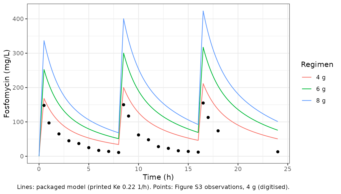
Replicate Figure 5: fitted time-kill curves
The points below are the authors’ fitted lines of Figure 5, digitised by the maintainers at the times where each line is clearly resolved. They are compared with the packaged model (printed Ke) and with the same model at Ke = 0.42 1/h.
fig5 <- read.table(header = TRUE, text = "
strain lzd fof time y
ATCC 4 0 4 5.8
ATCC 4 0 12 5.9
ATCC 4 0 24 6.1
ATCC 8 0 8 5.6
ATCC 8 0 24 5.55
ATCC 0 4 3 4.9
ATCC 0 4 8 7.5
ATCC 0 4 24 8.2
ATCC 0 8 5 4.5
ATCC 0 8 8 5.8
ATCC 0 8 12 6.3
ATCC 0 8 16 7.7
ATCC 4 4 2 5.3
ATCC 4 4 8 4.95
ATCC 4 4 24 4.6
ATCC 8 6 2 5.0
ATCC 8 6 8 4.0
ATCC 8 6 12 3.8
ATCC 8 6 24 3.65
No1 4 0 8 6.9
No1 4 0 24 8.5
No1 8 0 4 5.4
No1 8 0 24 4.95
No1 0 4 6 4.0
No1 0 4 12 5.3
No1 0 4 24 8.15
No1 0 6 7 3.8
No1 0 6 12 4.6
No1 0 6 24 7.8
No1 4 4 4 4.3
No1 4 4 12 3.45
No1 4 4 24 3.25
No1 8 6 4 3.8
No1 8 6 8 3.2
No1 8 6 24 2.65
No2 8 0 4 5.2
No2 8 0 24 8.2
No2 12 0 6 5.0
No2 12 0 24 4.9
No2 0 6 3 4.6
No2 0 6 8 6.5
No2 0 6 16 7.5
No2 0 6 24 8.0
No2 0 8 4 4.0
No2 0 8 8 5.5
No2 0 8 16 6.7
No2 0 8 24 7.5
No2 8 6 4 4.4
No2 8 6 12 4.0
No2 8 6 24 3.75
No2 12 8 2 4.7
No2 12 8 10 3.6
No2 12 8 24 3.4
No6 8 0 4 5.1
No6 8 0 24 4.87
No6 12 0 8 4.6
No6 12 0 24 4.4
No6 0 6 3 5.0
No6 0 6 8 6.9
No6 0 6 24 8.5
No6 0 8 4 4.7
No6 0 8 8 5.95
No6 0 8 16 7.5
No6 8 6 4 4.4
No6 8 6 12 3.9
No6 8 6 24 3.8
No6 12 8 4 4.0
No6 12 8 12 3.3
No6 12 8 24 3.2
") |>
  dplyr::mutate(
    strain = dplyr::recode(strain, ATCC = "ATCC 29212", No1 = "No. 1", No2 = "No. 2", No6 = "No. 6"),
    arm = arm_label(lzd, fof),
    therapy = ifelse(lzd > 0 & fof > 0, "combination", "monotherapy")
  )
stopifnot(nrow(fig5) == 69L, all(fig5$strain %in% strains$strain))
arms <- fig5 |>
  dplyr::distinct(strain, lzd, fof, arm, therapy) |>
  dplyr::bind_rows(tidyr::expand_grid(
    strain = strains$strain, lzd = 0, fof = 0, arm = "Control", therapy = "control"
  ))
curves <- dplyr::bind_rows(lapply(c(0.22, 0.42), function(ke) {
  dplyr::bind_rows(lapply(seq_len(nrow(arms)), function(i) {
    m <- with_ini(mods[[arms$strain[i]]], lkel = log(ke))
    sim_arm(m, arms$lzd[i], arms$fof[i]) |>
      dplyr::select(time, log_cfu) |>
      dplyr::mutate(
        strain = arms$strain[i], lzd = arms$lzd[i], fof = arms$fof[i],
        arm = arms$arm[i], therapy = arms$therapy[i], ke = ke
      )
  }))
}))
scored <- fig5 |>
  dplyr::inner_join(curves, by = c("strain", "lzd", "fof", "arm", "therapy", "time"), relationship = "many-to-many")
stopifnot(nrow(scored) == 2L * nrow(fig5))
rmse <- scored |>
  dplyr::group_by(ke, therapy) |>
  dplyr::summarise(rmse = sqrt(mean((log_cfu - y)^2)), n = dplyr::n(), .groups = "drop")
rmse_strain <- scored |>
  dplyr::group_by(ke, therapy, strain) |>
  dplyr::summarise(rmse = sqrt(mean((log_cfu - y)^2)), .groups = "drop") |>
  tidyr::pivot_wider(names_from = strain, values_from = rmse)
rmse |>
  dplyr::left_join(rmse_strain, by = c("ke", "therapy")) |>
  dplyr::rename("Ke (1/h)" = ke, "Arms" = therapy, "RMSE, all strains (log10 CFU/mL)" = rmse, "Points" = n) |>
knitr::kable(digits = 2, caption = "Root-mean-square difference between the packaged model and the digitised Figure 5 fitted lines.")| Ke (1/h) | Arms | RMSE, all strains (log10 CFU/mL) | Points | ATCC 29212 | No. 1 | No. 2 | No. 6 |
|---|---|---|---|---|---|---|---|
| 0.22 | combination | 2.95 | 25 | 2.57 | 2.55 | 3.26 | 3.39 |
| 0.22 | monotherapy | 0.58 | 44 | 0.47 | 0.24 | 0.89 | 0.48 |
| 0.42 | combination | 2.77 | 25 | 2.05 | 2.57 | 3.32 | 3.06 |
| 0.42 | monotherapy | 0.23 | 44 | 0.27 | 0.22 | 0.22 | 0.18 |
rm_of <- function(k, th) rmse$rmse[rmse$ke == k & rmse$therapy == th]
# Monotherapy reproduces the published fits with the printed parameters
# (realised 0.58 log10; 0.23 at Ke 0.42). A mis-transcribed Emax, EC50, Hill or
# growth parameter moves the affected curves by >1 log10 and fails this.
stopifnot(rm_of(0.22, "monotherapy") < 0.75, rm_of(0.42, "monotherapy") < 0.35)
# Recorded deviation: the combination arms do not reproduce (realised 2.95
# log10 at the printed Ke, 2.77 at 0.42). If this fails, the combination term
# has changed and the caution at the top of this article must be revisited.
stopifnot(rm_of(0.22, "combination") > 1.5, rm_of(0.42, "combination") > 1.5)
# Control growth reaches the stationary-phase maximum by 24 h.
ctl24 <- curves |> dplyr::filter(arm == "Control", time == 24, ke == 0.22)
bmax <- sapply(strains$strain, function(s) mods[[s]]$theta[["log10cfumax"]])
stopifnot(all(abs(ctl24$log_cfu - bmax[ctl24$strain]) < 0.05))
curves |>
  dplyr::filter(ke == 0.22) |>
  ggplot(aes(time, log_cfu, colour = arm)) +
  geom_line() +
  geom_point(data = fig5, aes(y = y), size = 2) +
  facet_grid(strain ~ therapy) +
  coord_cartesian(ylim = c(0, 9)) +
  labs(
    x = "Time (h)", y = "Viable count (log10 CFU/mL)", colour = "Arm",
    title = "Figure 5 - packaged model (lines) vs published fitted lines (points)",
    caption = "Replicates Figure 5 of Mao 2021. Printed Ke 0.22 1/h."
  ) +
  theme_bw() +
  theme(legend.position = "bottom") +
  guides(colour = guide_legend(ncol = 3))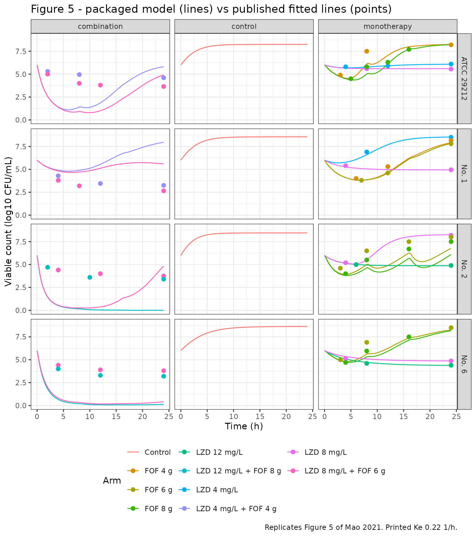
The monotherapy panels follow the published curves: linezolid is bacteriostatic, fosfomycin kills over the first 4-8 h and the count regrows to the stationary phase by 24 h (the regrowth is somewhat later with the printed Ke because fosfomycin accumulates). In the combination panels the published curves fall to a plateau of ~3-4.5 log10 CFU/mL with no regrowth. The packaged model departs from them in a strain-dependent way: for ATCC 29212 and the lower combination for No. 2 it drives the count to ~1 log10 or below within 6-8 h and then regrows as the adaptive-resistance factor rises; for No. 6 and the higher combination for No. 2 it sterilises; and for No. 1, whose interaction exponent is negative, it produces little kill and regrows.
Interaction equation checks
# 1. The encoded Equation 5 reduces to the single drug's effect: monotherapy
#    curves are unchanged when the interaction exponent is set to zero.
for (s in strains$strain) {
  m0 <- with_ini(mods[[s]], inter = 0)
  for (a in list(c(8, 0), c(0, 6))) {
    d <- max(abs(sim_arm(mods[[s]], a[1], a[2])$log_cfu - sim_arm(m0, a[1], a[2])$log_cfu))
    stopifnot(d < 1e-8)
  }
}
# 2. The form printed in the paper multiplies a monotherapy effect by 2^int.
inter_printed <- sapply(strains$strain, function(s) mods[[s]]$theta[["inter"]])
knitr::kable(
  data.frame(
    strain = strains$strain,
    int = unname(inter_printed),
    `monotherapy effect multiplier under the printed form (2^int)` = round(2^inter_printed, 2),
    check.names = FALSE
  ),
  row.names = FALSE,
  caption = "Why the printed Equation 5 is not used: it would scale every monotherapy kill rate by these factors, which the monotherapy fits above (multiplier 1) contradict."
)| strain | int | monotherapy effect multiplier under the printed form (2^int) |
|---|---|---|
| ATCC 29212 | 1.29 | 2.45 |
| No. 1 | -1.96 | 0.26 |
| No. 2 | 1.37 | 2.58 |
| No. 6 | 2.08 | 4.23 |
Figure 7: model-predicted regimens
The paper’s Results report the following predictions from Figure 7. The packaged model’s change in log10 CFU/mL from the 6 log10 inoculum at 24 h is shown for comparison. These are not gated; they illustrate the combination gap described above.
claims <- tibble::tribble(
  ~strain, ~lzd, ~fof, ~paper,
  "No. 2", 24, 0,  "bacteriostatic only, no bactericidal effect",
  "No. 2", 18, 10, "4 log10 reduction at 24 h",
  "No. 2", 24, 10, "greater than 5 log10 reduction at 24 h",
  "No. 6", 16, 6,  "greater than 4 log10 reduction at 24 h",
  "No. 1", 8,  2,  "3 log10 reduction at 24 h"
)
claims$model <- vapply(seq_len(nrow(claims)), function(i) {
  r <- sim_arm(mods[[claims$strain[i]]], claims$lzd[i], claims$fof[i], times = 24)
  r$log_cfu[r$time == 24] - 6
}, numeric(1))
claims |>
  dplyr::mutate(arm = arm_label(lzd, fof)) |>
  dplyr::select(strain, arm, paper, model) |>
  dplyr::rename(
    "Strain" = strain, "Regimen" = arm, "Paper (Results, Figure 7)" = paper,
    "Model change at 24 h (log10 CFU/mL)" = model
  ) |>
knitr::kable(digits = 2)| Strain | Regimen | Paper (Results, Figure 7) | Model change at 24 h (log10 CFU/mL) |
|---|---|---|---|
| No. 2 | LZD 24 mg/L | bacteriostatic only, no bactericidal effect | -1.13 |
| No. 2 | LZD 18 mg/L + FOF 10 g | 4 log10 reduction at 24 h | -6.00 |
| No. 2 | LZD 24 mg/L + FOF 10 g | greater than 5 log10 reduction at 24 h | -6.00 |
| No. 6 | LZD 16 mg/L + FOF 6 g | greater than 4 log10 reduction at 24 h | -5.82 |
| No. 1 | LZD 8 mg/L + FOF 2 g | 3 log10 reduction at 24 h | -0.48 |
Linezolid monotherapy reproduces the bacteriostatic prediction. The combination predictions do not: for strains No. 2 and No. 6 the model sterilises (about -6 log10), and for strain No. 1, whose interaction exponent is negative, it predicts little net kill rather than 3 log10.
Figure 6 (external validation, ATCC 29212 with linezolid 12 mg/L + fosfomycin 8 g) is not replicated quantitatively; the authors report that their own prediction under-estimated the observed kill by about 1 log10.
Assumptions and deviations
-
Combination term (Equation 5). Encoded in the form
of the cited source (Mohamed et al. 2016, reference 17), with the other
drug’s effect in each bracket. The printed form (same drug in each
bracket) is treated as a transcription error because it multiplies
monotherapy effects by
2^int(table above), which the paper’s monotherapy fits rule out. Neither form, an additive form, the printed form divided by2^int, nor a per-strain re-estimate ofintreproduces the published combination curves; the maintainers found the best achievable per-strain RMSE was 0.6-2.2 log10 withintvalues unrelated to those printed. The defect is therefore structural and is not described in the paper. The printed Table 3 values are encoded unchanged, and the combination arms should not be relied on to reproduce the paper. -
Fosfomycin Ke. Supplemental Table S1 prints Ke =
0.22 1/h and the models use it. The in-system targets stated in the
Methods (t1/2 beta 3.3 h, AUC0-8 383 mg*h/L, Cmax 160.2 mg/L at 4 g)
each back-solve to Ke = 0.42 / 0.42 / 0.43 1/h, and the Figure S3
observations and predicted line follow Ke ~0.42; a 4-to-2 digit misprint
is likely. Simulating with
ini(lkel = log(0.42))improves the monotherapy agreement from 0.58 to 0.23 log10 RMSE. No correction notice was found as of 2026-10-16. - V2. Table S1 also prints V2 = 10.26 L, which is close to but not equal to V1 * K12 / K21 = 10.49 L. The models use the rate-constant parameterisation (Ke, V1, K12, K21), in which V2 is not needed.
- Log-scale bacterial state. The paper does not say whether B is the count or its log10. Bmax is reported in log10 CFU/mL and the control curves reach ~8 log10 by 4 h, which a growth rate of ~0.45 1/h can only do on the log scale; the models treat B as log10 CFU/mL.
- Adaptive resistance. Equation 4 is applied literally: the concentration is the current concentration and t is the time since the start of the experiment, so the factor is not a state and does not decay when the concentration falls.
-
Sigmoid Emax algebra. Equation 3 is evaluated as
Emax / (1 + (alpha * EC50 / C)^Hill), which is algebraically identical and avoids floating-point overflow with the printed Hill coefficients of 50 and - Values at a bound. Several adaptation rates are printed as 0.0001 and strain No. 1 has a linezolid Hill coefficient of 187; these look like estimates at a bound but are encoded as printed.
- Initial inoculum. Not estimated; fixed at the nominal 6 log10 CFU/mL stated in the Methods.
- Residual error and variability. Not reported (the paper shows only goodness-of-fit and VPC plots). The additive residual SD is fixed at 0 and there is no between-replicate variability, so the VPC of Figure 4 is not replicated.
-
Interaction parameter name. The paper’s
intis a reserved word in the generated C code, so the models call itinter(the name also used inMohamed_2016_colistin_meropenem). - Digitised data. The Figure 5 fitted-line points and the Figure S3 concentrations were digitised by the maintainers from the published figures.