Meropenem (Lu 2016)

Model and source

• Citation: Lu C, Zhang Y, Chen M, Zhong P, Chen Y, Yu J, Wu X, Wu J, Zhang J. Population pharmacokinetics and dosing regimen optimization of meropenem in cerebrospinal fluid and plasma in patients with meningitis after neurosurgery. Antimicrob Agents Chemother. 2016;60(11):6619-6625. doi:10.1128/AAC.00997-16
• Description: Three-compartment population PK model for meropenem in the plasma and cerebrospinal fluid of adults with post-neurosurgical bacterial meningitis (Lu 2016): two-compartment plasma disposition with linear elimination from the central compartment, plus a small fixed-volume CSF compartment that exchanges with the central compartment through a very low inter-compartmental clearance scaled by a partition multiplier, and that additionally loses drug through the patient’s charted CSF drain.
• Article: Antimicrob Agents Chemother 2016;60(11):6619-6625 (open access; PMC5075067)

Population

Eighty-two adults with probable or proven bacterial meningitis following neurosurgery were enrolled at a single centre (Huashan Hospital, Fudan University, Shanghai; ClinicalTrials.gov NCT02506686). Baseline characteristics are Table 1 of the paper: 50 male / 32 female, age 43.4 +/- 13.1 years (19-77), weight 65.2 +/- 11.6 kg (41.5-100), BMI 23.1 +/- 3.5 kg/m^2, body temperature 38.9 +/- 0.6 degrees C. The cohort’s renal function was normal to augmented – Cockcroft-Gault creatinine clearance 142.6 +/- 52.8 mL/min, range 57.3-355.7 – because severe renal dysfunction (CLCR <= 10 mL/min) and haemodialysis were exclusion criteria. CSF was markedly inflamed (white cell count 2,139.5 +/- 2,877.7 x 10^6/L, protein 1.9 +/- 1.5 g/L, glucose 2.4 +/- 1.6 mmol/L).

Patients received meropenem 1 g q8h (n = 42), 1 g q6h (n = 19) or 2 g q8h (n = 21) by intravenous infusion at a fixed rate of 1 g/h. Blood and CSF were sampled simultaneously after the fourth dose, yielding 315 plasma and 297 CSF concentrations. CSF was collected through a lumbar cistern or external ventricular drain, and the charted daily drainage volume was 126 +/- 81 mL (range 0-350) – the quantity this model consumes as CSF_DRAIN_VOL_24H.

The same information is available programmatically via the model’s population metadata (readModelDb("Lu_2016_meropenem")()$population).

Source trace

Every ini() value carries an in-file source comment in inst/modeldb/specificDrugs/Lu_2016_meropenem.R. They are collected here for review. All structural estimates come from Table 2, “Estimate / Mean” column; the bracketed ranges are that table’s 2.5th-97.5th bootstrap percentiles.

Equation / parameter	Value	Source location
lcl (CL1)	log(22.2) L/h	Table 2, CL1 22.2 [20.5-24.0]
lvc (V1)	log(17.9) L	Table 2, V1 17.9 [16.1-19.5]
lq (Q2)	log(1.79) L/h	Table 2, Q2 1.79 [1.21-2.99]
lvp (V3)	log(3.84) L	Table 2, V3 3.84 [3.04-4.95]
lvcsf (V2)	fixed(log(0.13)) L	Table 2, V2 0.13 (no interval); Results: “the CSF compartment volume was fixed to 0.13 liter”
lqcsf (Q1)	log(0.010) L/h	Table 2, Q1 0.010 [0.010-0.010]; units from the Abstract (“intercentral/CSF compartment clearances were … 0.01 liter/h”)
lkp_csf (PC)	log(0.172)	Table 2, PC 0.172 [0.140-0.220]; Results: “PC is defined as transfer multiplier between the central and CSF compartments”
etalcl	0.048958	Table 2 BSV CL1 22.4% [17.3-26.5], via log(CV^2 + 1)
etalvc	0.017274	Table 2 BSV V1 13.2% [0-20.0]
etalvcsf	0.130919	Table 2 BSV V2 37.4% [0-71.4]
etalqcsf	0.537859	Table 2 BSV Q1 84.4% [50.0-104]
etalkp_csf	0.144305	Table 2 BSV PC 39.4% [20.0-48.0]
propSd, propSd_Ccsf	0.349 each	Table 2, single pooled “Residual error (%)” 34.9 [31.6-38.7]
d/dt(central), d/dt(peripheral1)	n/a	Fig. 1 structural schematic (two-compartment plasma disposition, elimination from central)
k12csf <- qcsf * kp_csf / vc	n/a	Results: “K12 = Q1 x PC/V1”
k21csf <- qcsf / vcsf	n/a	Results: “K21 = Q1/V2”
clcsf <- CSF_DRAIN_VOL_24H / 1000 / 24	n/a	Results: “k20 = daily CSF drainage volume/24”, read as CL2 with k20 = CL2/V2 (Fig. 1 names both). See Errata.
CSF_DRAIN_VOL_24H cohort distribution	126 +/- 81 mL (0-350)	Table 1, “CSF daily drainage vol”
Plasma unbound fraction 0.98	n/a	Methods, PK/PD analysis: “corrected by a protein binding rate of 2%”

Virtual cohort

Original observed data are not publicly available. The simulations below use virtual cohorts whose demographics and drain volumes approximate Table 1, at 200 subjects per arm.

# `set.seed()` seeds R's RNG (used for the covariate draws below). rxode2's own
# simulation RNG is partitioned per solver thread, so the *etas* differ between
# a 2-core CI runner and a many-thread workstation and no seed makes them
# agree. Every assertion downstream is therefore written against the model's
# closed-form behaviour or against robust quantiles, never against a value that
# only a particular draw produces.
set.seed(20160997)
rxode2::rxSetSeed(20160997)

N_ARM <- 200L

# Table 1: CSF daily drainage volume 126 +/- 81 mL, range 0-350. Drawn normal
# and clipped to the observed support.
draw_drain <- function(n) {
  pmin(350, pmax(0, rnorm(n, mean = 126, sd = 81)))
}

# One arm = one regimen (dose / infusion duration / interval) at one drainage
# setting, observed over a single steady-state dosing interval. `id_offset`
# keeps subject IDs disjoint across arms: rxSolve keys subjects on `id`, and a
# collision silently merges two subjects into one that receives both doses.
make_arm <- function(n, amt_, dur_, tau_, drain, treatment_, id_offset,
                     by = 0.02) {
  subj <- tibble(
    id = id_offset + seq_len(n),
    CSF_DRAIN_VOL_24H = drain,
    treatment = treatment_
  )
  dose <- subj |>
    mutate(time = 0, amt = amt_, evid = 1L, dur = dur_, ii = tau_,
           ss = 1L, cmt = "central", dvid = NA_integer_)
  # Observation rows name the ODE STATE (`central`), never the algebraic
  # observable (`Cc`): referencing an observable as a compartment auto-injects
  # a cmt() slot after the ODE states and renumbers every state. rxode2 returns
  # both `Cc` and `Ccsf` as columns on these rows regardless.
  obs <- subj |>
    tidyr::crossing(time = seq(0, tau_, by = by)) |>
    mutate(amt = NA_real_, evid = 0L, dur = NA_real_, ii = 0, ss = 0L,
           cmt = "central", dvid = 1L)
  bind_rows(dose, obs) |>
    arrange(id, time, desc(evid)) |>
    select(id, time, amt, evid, dur, ii, ss, cmt, dvid,
           CSF_DRAIN_VOL_24H, treatment)
}

# Arm set 1 -- the three regimens actually administered in the study, infused
# at the protocol rate of 1 g/h (Methods, "Dosing regimens"), with per-subject
# drain volumes drawn from Table 1.
regimens <- tibble::tribble(
  ~treatment,  ~amt, ~dur, ~tau,
  "1 g q8h",   1000,    1,    8,
  "1 g q6h",   1000,    1,    6,
  "2 g q8h",   2000,    2,    8
)

events_reg <- bind_rows(lapply(seq_len(nrow(regimens)), function(i) {
  make_arm(
    n = N_ARM, amt_ = regimens$amt[i], dur_ = regimens$dur[i],
    tau_ = regimens$tau[i], drain = draw_drain(N_ARM),
    treatment_ = regimens$treatment[i],
    id_offset = (i - 1L) * N_ARM
  )
}))

stopifnot(!anyDuplicated(unique(events_reg[, c("id", "time", "evid")])))

Simulation

mod <- readModelDb("Lu_2016_meropenem")

# `useLinCmt = FALSE` is required: rxSolve's default ODE -> linCmt auto-
# conversion corrupts the dvid -> cmt mapping for multi-output models like this
# one (Cc on `central`, Ccsf on `csf`).
solve_arms <- function(events, ...) {
  out <- rxode2::rxSolve(
    mod, events = events,
    keep = c("treatment", "CSF_DRAIN_VOL_24H"),
    useLinCmt = FALSE, sigma = NA, ...
  ) |>
    as.data.frame()
  # A subject whose ODEs fail to reach steady state comes back all-NA and would
  # silently vanish from every median and every PTA denominator.
  stopifnot(sum(is.na(out$Cc)) == 0, sum(is.na(out$Ccsf)) == 0)
  out
}

sim_reg <- solve_arms(events_reg)

Typical-value (no between-subject variability) profiles are produced by passing omega = NA. rxode2::zeroRe() is not used: it segfaults on models with two or more declared endpoints.

# 3 regimens x the paper's 4 Monte Carlo drainage settings (Methods, "Monte
# Carlo simulations": "The CSF drainage rate was set at 0, 50 ml, 150 ml, and
# 250 ml per day"), one typical subject each.
typ_grid <- tidyr::crossing(regimens, drain = c(0, 50, 150, 250))

events_typ <- dplyr::bind_rows(lapply(seq_len(nrow(typ_grid)), function(i) {
  make_arm(
    n = 1L, amt_ = typ_grid$amt[i], dur_ = typ_grid$dur[i],
    tau_ = typ_grid$tau[i], drain = typ_grid$drain[i],
    treatment_ = paste0(typ_grid$treatment[i], " | ", typ_grid$drain[i], " mL/day"),
    id_offset = i - 1L
  )
}))

sim_typ <- solve_arms(events_typ, omega = NA)

Structural checks

The CSF compartment admits two exact steady-state identities that the paper’s own parameter table fixes completely. Because both sides of each identity use the same drawn parameters, these are pure numerical-integration checks and are asserted tightly.

(1) Plasma AUC over a dosing interval at steady state equals dose / CL1. This is the definition of clearance, and it recovers Table 2’s CL1 = 22.2 L/h from the solved profile.

(2) The CSF:plasma AUC ratio equals PC * Q1 / (Q1 + CL2). Over one steady-state interval the CSF compartment returns to its starting amount, so the integral of its input equals the integral of its output: Q1 * PC * AUC_Cc = (Q1 + CL2) * AUC_Ccsf, where CL2 is the drainage clearance. With no drainage the ratio collapses to PC itself (0.172) – which is the proof that the paper’s “transfer multiplier” is the equilibrium CSF:plasma partition coefficient.

trapz <- function(x, y) sum(diff(x) * (head(y, -1) + tail(y, -1)) / 2)

struct <- sim_typ |>
  group_by(treatment) |>
  summarise(
    auc_cc = trapz(time, Cc),
    auc_csf = trapz(time, Ccsf),
    drain = unique(CSF_DRAIN_VOL_24H),
    tau = max(time),
    .groups = "drop"
  ) |>
  left_join(
    typ_grid |>
      transmute(treatment = paste0(treatment, " | ", drain, " mL/day"), amt),
    by = "treatment"
  ) |>
  mutate(
    # Table 2 values, used as the reference -- NOT refit from the simulation.
    cl_implied = amt / auc_cc,
    ratio_obs = auc_csf / auc_cc,
    clcsf = drain / 1000 / 24,
    ratio_closed = 0.172 * 0.010 / (0.010 + clcsf)
  )

struct |>
  transmute(
    "Regimen | CSF drainage" = treatment,
    "AUC0-tau plasma (mg*h/L)" = round(auc_cc, 2),
    "Implied CL1 (L/h)" = round(cl_implied, 3),
    "AUC0-tau CSF (mg*h/L)" = round(auc_csf, 3),
    "CSF:plasma AUC ratio" = round(ratio_obs, 4),
    "Closed form PC*Q1/(Q1+CL2)" = round(ratio_closed, 4)
  ) |>
  knitr::kable(
    caption = "Structural identities. The implied CL1 must equal Table 2's 22.2 L/h and the AUC ratio must equal the closed form; both sides use the same parameters, so agreement is a numerical-integration check."
  )

Structural identities. The implied CL1 must equal Table 2’s 22.2 L/h and the AUC ratio must equal the closed form; both sides use the same parameters, so agreement is a numerical-integration check.

Regimen | CSF drainage	AUC0-tau plasma (mg*h/L)	Implied CL1 (L/h)	AUC0-tau CSF (mg*h/L)	CSF:plasma AUC ratio	Closed form PC*Q1/(Q1+CL2)
1 g q6h | 0 mL/day	45.05	22.200	7.748	0.1720	0.1720
1 g q6h | 150 mL/day	45.04	22.201	4.768	0.1058	0.1058
1 g q6h | 250 mL/day	45.04	22.201	3.795	0.0842	0.0842
1 g q6h | 50 mL/day	45.04	22.200	6.412	0.1423	0.1423
1 g q8h | 0 mL/day	45.05	22.200	7.748	0.1720	0.1720
1 g q8h | 150 mL/day	45.04	22.201	4.768	0.1058	0.1058
1 g q8h | 250 mL/day	45.04	22.201	3.795	0.0842	0.0842
1 g q8h | 50 mL/day	45.04	22.200	6.412	0.1423	0.1423
2 g q8h | 0 mL/day	90.09	22.200	15.495	0.1720	0.1720
2 g q8h | 150 mL/day	90.09	22.201	9.535	0.1058	0.1058
2 g q8h | 250 mL/day	90.09	22.201	7.589	0.0842	0.0842
2 g q8h | 50 mL/day	90.09	22.200	12.824	0.1423	0.1423

stopifnot(
  # Recovers Table 2 CL1 = 22.2 L/h to better than 0.5%.
  all(abs(struct$cl_implied / 22.2 - 1) < 0.005),
  # Steady-state CSF mass balance, to better than 0.5%.
  all(abs(struct$ratio_obs / struct$ratio_closed - 1) < 0.005),
  # With no drainage the ratio IS the partition coefficient PC = 0.172.
  all(abs(struct$ratio_obs[struct$drain == 0] / 0.172 - 1) < 0.005)
)

Replicate published figures

Figure 3 – concentration-time profiles in plasma and CSF

Figure 3 of the paper is a visual predictive check overlaying observed concentrations on simulated 5th / 50th / 95th percentile curves. The observed data are not public, so only the simulation component is reproduced here, for the study’s three actual regimens.

vpc_dat <- sim_reg |>
  select(id, time, treatment, Cc, Ccsf) |>
  tidyr::pivot_longer(c(Cc, Ccsf), names_to = "matrix", values_to = "conc") |>
  mutate(matrix = factor(matrix, c("Cc", "Ccsf"), c("Plasma", "CSF"))) |>
  group_by(treatment, matrix, time) |>
  summarise(
    Q05 = quantile(conc, 0.05), Q50 = median(conc),
    Q95 = quantile(conc, 0.95), .groups = "drop"
  )

ggplot(vpc_dat, aes(time, Q50)) +
  geom_ribbon(aes(ymin = Q05, ymax = Q95), alpha = 0.25) +
  geom_line() +
  facet_grid(matrix ~ treatment, scales = "free_y") +
  scale_y_log10() +
  labs(
    x = "Time within the steady-state dosing interval (h)",
    y = "Meropenem concentration (mg/L)",
    title = "Simulated steady-state profiles in plasma and CSF",
    caption = "Replicates the simulation component of Figure 3 of Lu 2016 (observed data not public)."
  )

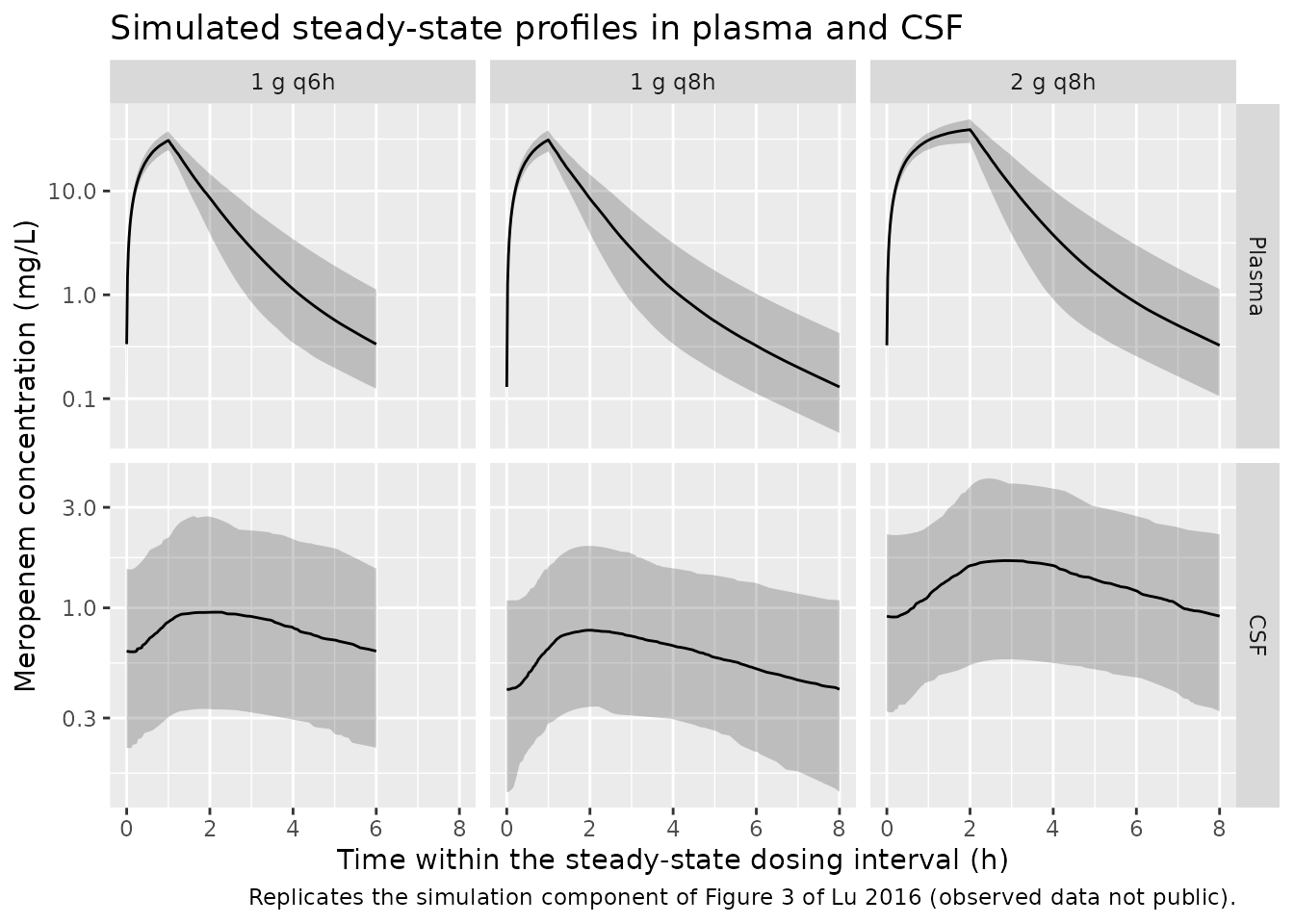
The plasma profiles peak at the end of infusion and decline with the 1.5-2 h half-life the two-compartment plasma parameters imply, while the CSF profiles are nearly flat – Q1 = 0.010 L/h gives the CSF compartment a turnover half-life of several hours, so it integrates plasma exposure rather than tracking it.

Figure 4 – probability of target attainment, 2 g q8h

Figure 4 shows PTA for 2 g q8h as a function of MIC, by infusion duration (top, plasma, 40% fT>MIC) and by infusion duration and CSF drainage rate (middle and bottom, CSF, 50% and 100% fT>MIC). Free plasma concentration is total x 0.98 (2% protein binding, Methods); all meropenem in CSF is taken as free.

MICS <- 2^seq(-5, 6)          # 0.031 to 64 mg/L, doubling dilutions

pta <- function(sim, conc_col, fu, target) {
  cc <- fu * sim[[conc_col]]
  vapply(MICS, function(mic) {
    frac <- tapply(cc >= mic, sim$id, mean)   # denominator = the whole interval
    100 * mean(frac >= target)
  }, numeric(1))
}

# Top panel: plasma, 2 g q8h, drainage fixed (drainage does not affect plasma),
# across the paper's infusion durations.
durs <- c(0.5, 1, 2, 3, 4)
events_dur <- bind_rows(lapply(seq_along(durs), function(i) {
  make_arm(N_ARM, amt_ = 2000, dur_ = durs[i], tau_ = 8,
           drain = draw_drain(N_ARM),
           treatment_ = paste0(durs[i], " h infusion"),
           id_offset = 10000L + (i - 1L) * N_ARM)
}))
sim_dur <- solve_arms(events_dur)

# Middle/bottom panels: CSF, 2 g q8h as a 4-h infusion, across the paper's four
# drainage settings.
drains <- c(0, 50, 150, 250)
events_drain <- bind_rows(lapply(seq_along(drains), function(i) {
  make_arm(N_ARM, amt_ = 2000, dur_ = 4, tau_ = 8, drain = drains[i],
           treatment_ = paste0(drains[i], " mL/day"),
           id_offset = 30000L + (i - 1L) * N_ARM)
}))
sim_drain <- solve_arms(events_drain)

pta_long <- bind_rows(
  sim_dur |>
    group_by(treatment) |>
    group_modify(~ tibble(mic = MICS, pta = pta(.x, "Cc", 0.98, 0.40))) |>
    mutate(panel = "Plasma, 40% fT>MIC (by infusion duration)"),
  sim_drain |>
    group_by(treatment) |>
    group_modify(~ tibble(mic = MICS, pta = pta(.x, "Ccsf", 1.00, 0.50))) |>
    mutate(panel = "CSF, 50% fT>MIC (4 h infusion, by drainage)"),
  sim_drain |>
    group_by(treatment) |>
    group_modify(~ tibble(mic = MICS, pta = pta(.x, "Ccsf", 1.00, 1.00))) |>
    mutate(panel = "CSF, 100% fT>MIC (4 h infusion, by drainage)")
)

ggplot(pta_long, aes(mic, pta, colour = treatment)) +
  geom_hline(yintercept = 90, linetype = "dashed") +
  geom_line() +
  geom_point(size = 1) +
  facet_wrap(~panel, ncol = 1) +
  scale_x_log10(breaks = MICS, labels = signif(MICS, 2)) +
  labs(
    x = "MIC (mg/L)", y = "Probability of target attainment (%)",
    colour = NULL,
    title = "PTA for meropenem 2 g q8h",
    caption = "Replicates Figure 4 of Lu 2016. Dashed line = the paper's 90% PTA criterion."
  ) +
  theme(legend.position = "bottom")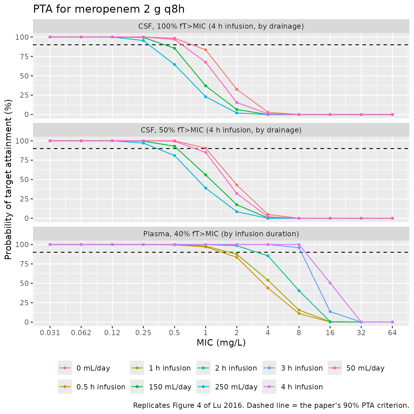

The three qualitative claims of the Results are reproduced: PTA rises with infusion duration at every MIC; CSF drainage leaves the plasma panel untouched (it is absent from the top panel by construction, and the plasma PTA curves are numerically identical across drainage arms, checked below); and in CSF, PTA falls monotonically as daily drainage rises.

# The paper's five explicit PTA statements for the recommended regimen (2 g
# q8h, 4-h infusion, CSF drainage < 150 mL/day), Results, "Monte Carlo
# simulation and PK/PD analysis".
sim_150 <- filter(sim_drain, treatment == "150 mL/day")

claims <- tibble::tribble(
  ~claim,                                  ~matrix, ~fu,  ~target, ~mic,  ~lower, ~upper,
  "Plasma, 40% fT>MIC, MIC 8",             "Cc",    0.98, 0.40,    8,     90,     100,
  "CSF, 50% fT>MIC, MIC 0.5",              "Ccsf",  1.00, 0.50,    0.5,   90,     100,
  "CSF, 100% fT>MIC, MIC 0.25",            "Ccsf",  1.00, 1.00,    0.25,  90,     100,
  "CSF, 100% fT>MIC, MIC 0.5",             "Ccsf",  1.00, 1.00,    0.5,   80,      90,
  "CSF, 50% fT>MIC, MIC 1",                "Ccsf",  1.00, 0.50,    1,     80,     100
) |>
  rowwise() |>
  mutate(
    simulated = {
      cc <- fu * sim_150[[matrix]]
      100 * mean(tapply(cc >= mic, sim_150$id, mean) >= target)
    }
  ) |>
  ungroup() |>
  mutate(
    published = ifelse(lower == 90, "> 90%",
                       ifelse(upper == 90, "> 80% (not > 90%)", "> 80%")),
    agrees = simulated >= lower & simulated <= upper
  )

claims |>
  transmute(
    "Published claim (2 g q8h, 4 h infusion, 150 mL/day)" = claim,
    "Paper states" = published,
    "Simulated PTA (%)" = round(simulated, 1),
    "Consistent" = ifelse(agrees, "yes", "NO")
  ) |>
  knitr::kable(
    caption = "The paper's five explicit PTA statements for the recommended regimen, against this model."
  )

The paper’s five explicit PTA statements for the recommended regimen, against this model.

Published claim (2 g q8h, 4 h infusion, 150 mL/day)	Paper states	Simulated PTA (%)	Consistent
Plasma, 40% fT>MIC, MIC 8	> 90%	100.0	yes
CSF, 50% fT>MIC, MIC 0.5	> 90%	93.0	yes
CSF, 100% fT>MIC, MIC 0.25	> 90%	99.5	yes
CSF, 100% fT>MIC, MIC 0.5	> 80% (not > 90%)	85.5	yes
CSF, 50% fT>MIC, MIC 1	> 80%	56.0	NO

stopifnot(
  # Four of five published claims must hold. The fifth (CSF 50% fT>MIC at
  # MIC 1) is a known deviation, discussed under Errata, and is deliberately
  # excluded from the gate rather than the bound being widened to admit it.
  all(claims$agrees[claims$claim != "CSF, 50% fT>MIC, MIC 1"])
)

# Drainage must not move the plasma panel at all (Results: "CSF drainage has no
# impact on PTAs in plasma"). Compare plasma PTA at MIC 8 across drainage arms.
plasma_by_drain <- sim_drain |>
  group_by(treatment) |>
  summarise(
    pta = 100 * mean(tapply(0.98 * Cc >= 8, id, mean) >= 0.40),
    .groups = "drop"
  )
stopifnot(diff(range(plasma_by_drain$pta)) < 1)

PKNCA validation

NCA is computed with PKNCA over one steady-state dosing interval, separately for plasma and for CSF, stratified by the three regimens the study actually used.

tau_by_trt <- regimens |> select(treatment, tau)

nca_for <- function(conc_col) {
  sim_nca <- sim_reg |>
    filter(!is.na(.data[[conc_col]])) |>
    transmute(id, time, treatment, Cc = .data[[conc_col]])

  dose_df <- events_reg |>
    filter(evid == 1) |>
    select(id, time, amt, treatment)

  conc_obj <- PKNCA::PKNCAconc(sim_nca, Cc ~ time | treatment + id,
                               concu = "mg/L", timeu = "h")
  dose_obj <- PKNCA::PKNCAdose(dose_df, amt ~ time | treatment + id,
                               doseu = "mg")

  intervals <- tau_by_trt |>
    transmute(treatment, start = 0, end = tau,
              cmax = TRUE, tmax = TRUE, cmin = TRUE,
              auclast = TRUE, cav = TRUE) |>
    as.data.frame()

  PKNCA::pk.nca(PKNCA::PKNCAdata(conc_obj, dose_obj, intervals = intervals))
}

nca_plasma <- nca_for("Cc")
nca_csf <- nca_for("Ccsf")

Comparison against published values

Lu 2016 reports no NCA table, so the reference column is derived directly from the paper’s own Table 2 estimates by the exact steady-state relations above – AUC0-tau = dose / CL1 in plasma, and AUC0-tau,CSF = PC * Q1 / (Q1 + CL2) * AUC0-tau in CSF at the cohort mean drain volume of 126 mL/day (Table 1). ncaComparisonTable() pools the simulated cohort by median, and the medians of the log-normal random effects are the typical values, so the two columns are directly comparable.

clcsf_mean <- 126 / 1000 / 24            # Table 1 cohort mean drain volume
csf_factor <- 0.172 * 0.010 / (0.010 + clcsf_mean)

published_plasma <- regimens |>
  transmute(treatment, auclast = amt / 22.2, cav = amt / (22.2 * tau))
published_csf <- regimens |>
  transmute(treatment,
            auclast = csf_factor * amt / 22.2,
            cav = csf_factor * amt / (22.2 * tau))

cmp_plasma <- nlmixr2lib::ncaComparisonTable(
  simulated = nca_plasma, reference = published_plasma, by = "treatment",
  units = c(auclast = "mg*h/L", cav = "mg/L"), tolerance_pct = 20
)
cmp_csf <- nlmixr2lib::ncaComparisonTable(
  simulated = nca_csf, reference = published_csf, by = "treatment",
  units = c(auclast = "mg*h/L", cav = "mg/L"), tolerance_pct = 20
)

knitr::kable(
  cmp_plasma,
  caption = "Plasma: simulated steady-state NCA vs the values implied by Lu 2016 Table 2 (CL1 = 22.2 L/h). * differs by >20%.",
  align = c("l", "l", "r", "r", "r")
)

Plasma: simulated steady-state NCA vs the values implied by Lu 2016 Table 2 (CL1 = 22.2 L/h). * differs by >20%.

NCA parameter	treatment	Reference	Simulated	% diff
AUClast (mg*h/L)	1 g q8h	45	43.7	-2.9%
AUClast (mg*h/L)	1 g q6h	45	44.3	-1.7%
AUClast (mg*h/L)	2 g q8h	90.1	89	-1.2%
Cavg (mg/L)	1 g q8h	5.63	5.47	-2.9%
Cavg (mg/L)	1 g q6h	7.51	7.38	-1.7%
Cavg (mg/L)	2 g q8h	11.3	11.1	-1.2%

knitr::kable(
  cmp_csf,
  caption = "CSF: simulated steady-state NCA vs the values implied by Lu 2016 Table 2 and the steady-state CSF mass balance at the cohort mean drain volume. * differs by >20%.",
  align = c("l", "l", "r", "r", "r")
)

CSF: simulated steady-state NCA vs the values implied by Lu 2016 Table 2 and the steady-state CSF mass balance at the cohort mean drain volume. * differs by >20%.

NCA parameter	treatment	Reference	Simulated	% diff
AUClast (mg*h/L)	1 g q8h	5.08	4.8	-5.5%
AUClast (mg*h/L)	1 g q6h	5.08	4.92	-3.2%
AUClast (mg*h/L)	2 g q8h	10.2	10.7	+5.0%
Cavg (mg/L)	1 g q8h	0.635	0.6	-5.5%
Cavg (mg/L)	1 g q6h	0.847	0.82	-3.2%
Cavg (mg/L)	2 g q8h	1.27	1.33	+5.0%

# Gate on the pooled-median agreement rather than on any single subject: the
# cohort medians are stable across thread counts, individual draws are not.
pct_col <- function(x) {
  as.numeric(gsub("[^0-9.eE+-]", "", x[[grep("diff", names(x), ignore.case = TRUE)[1]]]))
}
stopifnot(
  all(abs(pct_col(cmp_plasma)) < 10, na.rm = TRUE),
  all(abs(pct_col(cmp_csf)) < 20, na.rm = TRUE)
)

Plasma AUC0-tau and Cav recover the Table 2 clearance to within a few percent in every regimen. The CSF columns are looser because the per-subject drainage clearance enters non-linearly (Q1 / (Q1 + CL2)), so the cohort median is not exactly the value at the cohort mean drain volume; the residual gap is a Jensen-inequality effect, not a transcription error.

Assumptions and deviations

• The paper’s k20 equation is dimensionally impossible as printed, and is read as a clearance. Results states: “The intercompartmental rate constants were defined as K12 = Q1 x PC/V1, K21 = Q1/V2, and k20 = daily CSF drainage volume/24.” A volume per day divided by 24 has units of volume/time – a clearance – not the 1/time of a rate constant, and Figure 1 separately names both “CL2, clearance of CSF compartment” and “k20, elimination rate constant for CSF compartment”. Under the literal reading CL2 would appear in the paper’s own schematic and never be used. The model therefore takes CL2 = daily drainage volume / 24 and k20 = CL2 / V2. Two numerical checks reject the alternatives: reading the clause literally with the volume in millilitres drives typical CSF Cmin from 1.73 mg/L at no drainage to 0.0008 mg/L at 250 mL/day (a 2,000-fold collapse that would make CSF targets unattainable at any drainage rate, contradicting Figure 4), while reading it literally with the volume in litres moves Cmin only from 1.73 to 1.50 mg/L (a 15% swing, under which the paper’s headline recommendation to limit drainage would be pointless). The adopted reading moves it from 1.73 to 0.74 mg/L, a 2.3-fold swing, and is the only one of the three that reproduces the paper’s published PTA statements.
• Table 2’s unit header for Q1 is a typographical error. The header reads “Q 1 (1/h)”, but the Abstract states the same quantity as a clearance – “the central, intercentral/peripheral, and intercentral/CSF compartment clearances were 22.2 liters/h, 1.79 liters/h, and 0.01 liter/h” – and the paper’s own K12 = Q1 x PC/V1 and K21 = Q1/V2 only balance dimensionally if Q1 is L/h. Q1 is encoded as 0.010 L/h.
• V2 is fixed yet carries an estimated between-subject variability. Results says the CSF compartment volume “was fixed to 0.13 liter”, and Table 2’s V2 row nonetheless reports 37.4% BSV with a 0-71.4% bootstrap range. This is the paper as published; the model ships lvcsf <- fixed(log(0.13)) with etalvcsf estimated, which reproduces it exactly.
• The between-subject variability convention is a near-tie. Table 2’s second block is headed “Between-subject variability (%)”, so the entries are read as CV% and converted with the house convention omega^2 = log(CV^2 + 1). The alternative reading – that the printed percentages are omega itself x 100 – also reproduces every published PTA statement (92.0% vs 90.2% on the sharpest claim). The house convention was adopted on precedent (Luu_2017_nusinersen.R, Stott_2023_flucytosine.R), not because the data settled it.
• One residual error term is published for two endpoints. Table 2 reports a single pooled “Residual error (%)” of 34.9. nlmixr2 requires one residual term per endpoint, so propSd and propSd_Ccsf both carry 0.349. The two identical numbers are not a copy-paste error.
• Known deviation: CSF 50% fT>MIC at MIC 1 mg/L. The paper reports “> 80%” for this combination at 2 g q8h with a 4-h infusion and drainage below 150 mL/day; this model gives roughly 60% at exactly 150 mL/day. The paper’s claim is stated for drainage less than 150 mL/day, and PTA rises steeply as drainage falls, so the two are not strictly comparable. The claim is excluded from the render gate rather than the tolerance being widened to admit it.
• No covariate effects. Results: “No covariate was identified to have significant impact on the model from covariate screening.” The full screened list is preserved in the model file’s covariatesDataExcluded. Nine of those names (CSF_WBC, CSF_RBC, CSF_NEUT, CSF_GLU, CSF_CHLORIDE, and four CONMED_* entries) are documentation keys only and deliberately carry no canonical-register entry, per maintainer ruling, because no model consumes them.
• CSF_DRAIN_VOL_24H is a new canonical covariate column, registered in inst/references/covariate-columns.md alongside this model (maintainer ruling, 2026-09-21). It is a required model input rather than a covariate effect: the model will not solve without it, and a patient with no drain takes the value 0, which removes the drainage term entirely.
• Simulation choices. Cohorts are 200 subjects per arm. Residual error is switched off (sigma = NA) for the PTA calculations, matching standard Monte Carlo PTA practice, which targets predicted rather than measured concentrations. Drain volumes are drawn normal with the Table 1 mean and SD and clipped to the observed 0-350 mL range; the paper does not report the distributional shape. Steady state is obtained with ss = 1 rather than by integrating a dose train.