Meropenem (Cojutti 2020)
Source:vignettes/articles/Cojutti_2020_meropenem.Rmd
Cojutti_2020_meropenem.RmdModel and source
- Citation: Cojutti PG, Candoni A, Lazzarotto D, Fili C, Zannier M, Fanin R, Pea F. Population Pharmacokinetics of Continuous-Infusion Meropenem in Febrile Neutropenic Patients with Hematologic Malignancies: Dosing Strategies for Optimizing Empirical Treatment against Enterobacterales and P. aeruginosa. Pharmaceutics. 2020;12(9):785. doi:10.3390/pharmaceutics12090785
- Description: One-compartment IV population PK model for continuous-infusion meropenem in 61 adult febrile neutropenic patients with hematologic malignancies (Cojutti 2020). Pmetrics NPAG non-parametric fit; clearance is a linear function of CKD-EPI creatinine clearance (CL = theta1 + theta2 * CRCL, both terms with their own between-subject distribution) and volume carries no covariate. Age, height, weight and sex were screened but not retained.
- Article: https://doi.org/10.3390/pharmaceutics12090785 (open access)
Population
The data came from a prospective, monocentric, interventional study at the Santa Maria della Misericordia University-Hospital of Udine (Italy) in which febrile neutropenic adults with hematologic malignancies received meropenem by continuous infusion (CI) with real-time therapeutic drug monitoring (TDM) targeting a steady-state concentration (Css) of 8-16 mg/L. Treatment started with a 1 g loading dose over 30 min followed by 1 g q8h CI (CLCR >= 60 mL/min/1.73 m^2) or 0.5 g q6h CI (CLCR < 60), then was adjusted to the TDM result. Of 100 enrolled patients, 61 had adequate sampling and contributed 178 steady-state concentrations (median 3 TDM assessments per patient).
Cojutti 2020 Table 1: median age 55 years (IQR 54-60), 37 male / 24 female, median weight 77 kg (IQR 63-85), median CKD-EPI creatinine clearance 107.3 mL/min/1.73 m^2 (IQR 96.1-123.6), with 22.9% showing augmented renal clearance (ARC, CLCR >= 130). Underlying disease: acute myeloid leukemia 57.4%, lymphoma 19.7%, acute lymphocytic leukemia 18.0%, multiple myeloma 4.9%. Median CI meropenem dose 1 g q8h; median therapy 9 days.
The same information is available programmatically via
readModelDb("Cojutti_2020_meropenem")$population.
Source trace
Per-parameter origins are recorded inline in
inst/modeldb/specificDrugs/Cojutti_2020_meropenem.R.
| Equation / parameter | Value | Source location |
|---|---|---|
| Structure: one compartment, zero-order input, first-order elimination | – | Methods 2.2 |
cl = theta1 + theta2 * CRCL |
– | Results 3.2, Equation 1 |
lcl (theta1, CL at CRCL = 0) |
0.27 L/h | Table 2, Mean column (SD 0.13, median 0.20) |
e_crcl_cl (theta2, slope on CRCL) |
0.12 L/h per mL/min/1.73 m^2 | Table 2, Mean column (SD 0.03, median 0.13) |
lvc (V) |
21.88 L | Table 2, Mean column (SD 5.85, median 20.00) |
etalcl |
log(0.4853^2 + 1) = 0.2114 | Table 2, theta1 CV 48.53% |
etae_crcl_cl |
log(0.2744^2 + 1) = 0.0726 | Table 2, theta2 CV 27.44% |
etalvc |
log(0.2671^2 + 1) = 0.0689 | Table 2, V CV 26.71% |
addSd |
5 x 0.224 = 1.12 mg/L | Methods 2.2, assay C0 = 0.224 times gamma G = 5 |
propSd |
5 x 0.060 = 0.30 | Methods 2.2, assay C1 = 0.060 times gamma G = 5 |
CRCL covariate |
CKD-EPI, mL/min/1.73 m^2 | Methods 2.1 |
Typical-value check against the reported mean clearance
The paper reports a mean population clearance of 13.04 L/h (Results 3.2). The Table 2 mean coefficients evaluated at the cohort’s median CLCR reproduce it; the Table 2 median coefficients do not (0.20 + 0.13 x 107.3 = 14.15 L/h, +8.5%), which is one of the two reasons the mean column is used (the other is the Figure 4 replication below).
mod <- readModelDb("Cojutti_2020_meropenem")
ini_df <- rxode2::rxode(mod)$iniDf
#> ℹ parameter labels from comments will be replaced by 'label()'
theta <- setNames(ini_df$est, ini_df$name)
cl_median_crcl <- exp(theta[["lcl"]]) + theta[["e_crcl_cl"]] * 107.3
cl_median_crcl
#> [1] 13.146
stopifnot(abs(cl_median_crcl / 13.04 - 1) < 0.02)
Virtual cohorts
Two simulations are run.
- Monte Carlo renal-function classes (Figure 4 replication). The paper split CLCR into three classes – 50-89, 90-129 and >= 130 mL/min/1.73 m^2 – and simulated each regimen at 48 h without a loading dose. The class means and SDs it sampled from are not reported, so CLCR is drawn uniformly within each class (upper bound 170 for ARC, the right edge of the Figure 3 histogram). Each class is simulated at 1 g q8h CI; because the model is linear, Css for every other regimen is that Css scaled by the ratio of daily doses (checked below).
- Study cohort at the median regimen (1 g loading dose over 30 min, then 1 g q8h CI), with CLCR drawn log-normally around the Table 1 median 107.3 and a spread matching its IQR.
rxode2::rxSetSeed(20200819)
n_per_arm <- 200

class_def <- tibble::tibble(
  treatment = c("CLCR 50-89", "CLCR 90-129", "CLCR >=130"),
  lo = c(50, 90, 130),
  hi = c(89, 129, 170)
)

cov_class <- class_def |>
  dplyr::rowwise() |>
  dplyr::reframe(
    treatment = treatment,
    CRCL = stats::runif(n_per_arm, lo, hi)
  )

cov_study <- tibble::tibble(
  treatment = "Study cohort (1 g LD + 1 g q8h CI)",
  CRCL = 107.3 * exp(stats::rnorm(n_per_arm, 0, log(123.6 / 96.1) / 1.349))
)

covs <- dplyr::bind_rows(cov_class, cov_study) |>
  dplyr::mutate(id = dplyr::row_number())

tau <- 8
dose_mg <- 1000
rate_mgh <- dose_mg / tau
obs_times <- seq(0, 48, by = 0.5)

maint <- tidyr::expand_grid(id = covs$id, time = seq(0, 48 - tau, by = tau)) |>
  dplyr::mutate(amt = dose_mg, rate = rate_mgh, evid = 1L, cmt = "central")
loading <- covs |>
  dplyr::filter(grepl("Study", treatment)) |>
  dplyr::transmute(id, time = 0, amt = 1000, rate = 1000 / 0.5, evid = 1L, cmt = "central")
obs <- tidyr::expand_grid(id = covs$id, time = obs_times) |>
  dplyr::mutate(amt = NA_real_, rate = NA_real_, evid = 0L, cmt = "central")

events <- dplyr::bind_rows(maint, loading, obs) |>
  dplyr::left_join(covs, by = "id") |>
  dplyr::arrange(id, time, dplyr::desc(evid))
Simulation
sim <- rxode2::rxSolve(mod, events, keep = c("treatment", "CRCL")) |>
  as.data.frame()
#> ℹ parameter labels from comments will be replaced by 'label()'
sim |>
  dplyr::group_by(treatment, time) |>
  dplyr::summarise(
    med = stats::median(Cc), lo = stats::quantile(Cc, 0.05),
    hi = stats::quantile(Cc, 0.95), .groups = "drop"
  ) |>
  ggplot(aes(time, med)) +
  geom_ribbon(aes(ymin = lo, ymax = hi), alpha = 0.25) +
  geom_line() +
  geom_hline(yintercept = c(8, 16), linetype = "dashed") +
  facet_wrap(~treatment) +
  labs(x = "Time (h)", y = "Meropenem Cc (mg/L)")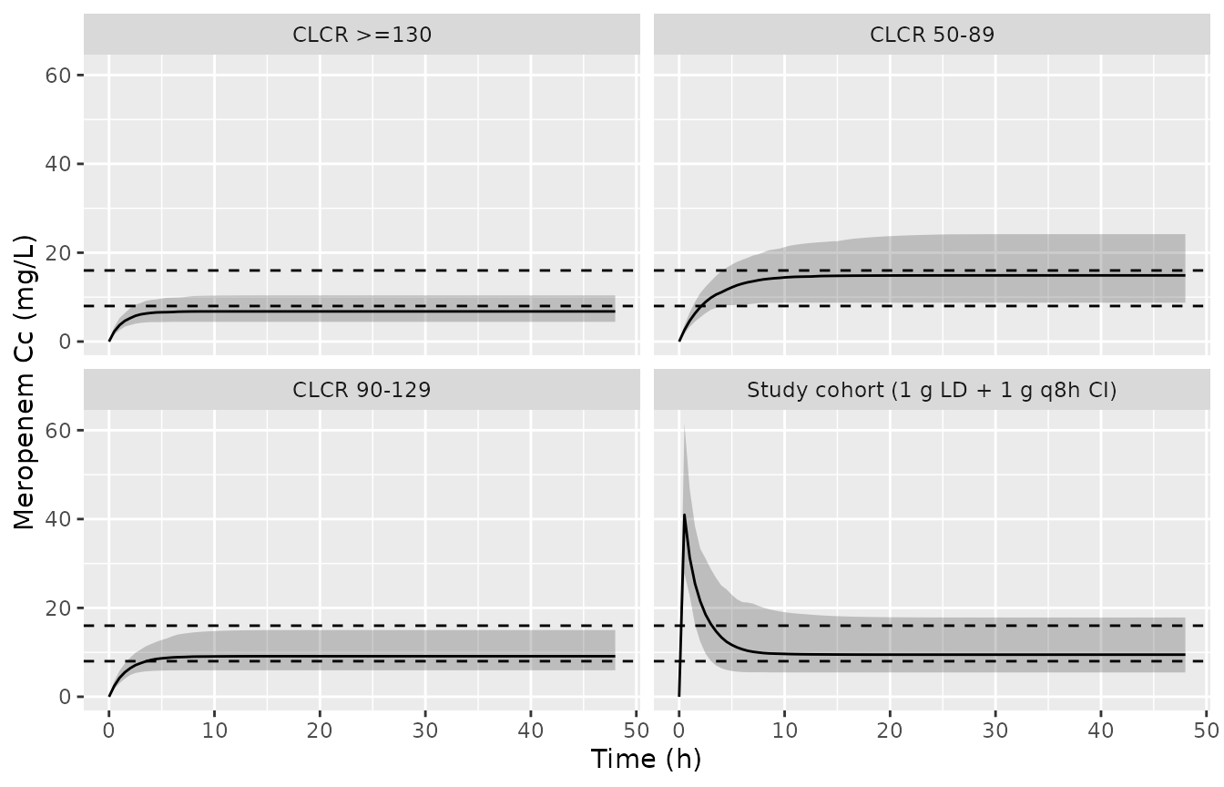
Simulated meropenem concentrations (median and 5th-95th percentiles) during 1 g q8h continuous infusion, by renal-function group. Dashed lines mark the TDM target band of 8-16 mg/L.
Solve matches the closed-form infusion solution
For a constant-rate infusion started at time zero with no loading
dose, the one-compartment solution is
C(t) = R / CL * (1 - exp(-kel * t)). Both sides use each
subject’s own drawn parameters, so the difference is pure numerical
error and the tolerance is tight. At 48 h this is Css = R / CL for all
but the slowest-clearing subjects, which also justifies scaling Css
linearly across regimens.
css <- sim |>
  dplyr::filter(time == 48) |>
  dplyr::mutate(
    c_closed = rate_mgh / cl * (1 - exp(-kel * time)),
    rel = Cc / c_closed - 1
  )
closed_chk <- css |> dplyr::filter(!grepl("Study", treatment))
summary(closed_chk$rel)
#>       Min.    1st Qu.     Median       Mean    3rd Qu.       Max.
#> -4.000e-15  0.000e+00  1.200e-14  1.401e-09  4.907e-11  7.119e-08
stopifnot(max(abs(closed_chk$rel)) < 1e-4)
Replicating Figure 4 (probability of target attainment)
Figure 4 of Cojutti 2020 plots the PTA of Css/MIC >= 4 and >= 1 at the EUCAST breakpoint of 2 mg/L (i.e. Css >= 8 and >= 2 mg/L) against the daily CI dose. The published points below were read from the figure by the maintainers.
regimens <- tibble::tibble(
  regimen = c("0.25 g q6h", "0.5 g q6h", "1 g q8h", "1 g q6h", "1.25 g q6h", "1.5 g q6h"),
  daily_g = 1:6
)

pta_sim <- css |>
  dplyr::filter(!grepl("Study", treatment)) |>
  tidyr::expand_grid(regimens) |>
  dplyr::mutate(css_reg = Cc * daily_g / 3) |>
  dplyr::group_by(treatment, daily_g) |>
  dplyr::summarise(
    pta4 = 100 * mean(css_reg >= 8),
    pta1 = 100 * mean(css_reg >= 2),
    .groups = "drop"
  )

pta_paper <- tibble::tribble(
  ~treatment,    ~daily_g, ~pta4_paper, ~pta1_paper,
  "CLCR 50-89",  1,  7,   100,
  "CLCR 50-89",  2,  65,  100,
  "CLCR 50-89",  3,  98,  100,
  "CLCR 50-89",  4,  100, 100,
  "CLCR 90-129", 1,  1,   93,
  "CLCR 90-129", 2,  19,  100,
  "CLCR 90-129", 3,  67,  100,
  "CLCR 90-129", 4,  95,  100,
  "CLCR 90-129", 5,  100, 100,
  "CLCR >=130",  1,  0,   67,
  "CLCR >=130",  2,  4,   100,
  "CLCR >=130",  3,  30,  100,
  "CLCR >=130",  4,  69,  100,
  "CLCR >=130",  5,  91,  100,
  "CLCR >=130",  6,  99,  100
)

pta_cmp <- pta_sim |>
  dplyr::inner_join(pta_paper, by = c("treatment", "daily_g"))

pta_cmp |>
  dplyr::rename(
    "CLCR class" = treatment, "Daily dose (g)" = daily_g,
    "PTA Css/MIC>=4, simulated (%)" = pta4, "PTA Css/MIC>=4, Figure 4 (%)" = pta4_paper,
    "PTA Css/MIC>=1, simulated (%)" = pta1, "PTA Css/MIC>=1, Figure 4 (%)" = pta1_paper
  ) |>
knitr::kable(digits = 1)| CLCR class | Daily dose (g) | PTA Css/MIC>=4, simulated (%) | PTA Css/MIC>=1, simulated (%) | PTA Css/MIC>=4, Figure 4 (%) | PTA Css/MIC>=1, Figure 4 (%) |
|---|---|---|---|---|---|
| CLCR 50-89 | 1 | 5.5 | 100.0 | 7 | 100 |
| CLCR 50-89 | 2 | 75.5 | 100.0 | 65 | 100 |
| CLCR 50-89 | 3 | 97.0 | 100.0 | 98 | 100 |
| CLCR 50-89 | 4 | 100.0 | 100.0 | 100 | 100 |
| CLCR 90-129 | 1 | 0.0 | 94.0 | 1 | 93 |
| CLCR 90-129 | 2 | 16.0 | 100.0 | 19 | 100 |
| CLCR 90-129 | 3 | 64.5 | 100.0 | 67 | 100 |
| CLCR 90-129 | 4 | 94.0 | 100.0 | 95 | 100 |
| CLCR 90-129 | 5 | 99.5 | 100.0 | 100 | 100 |
| CLCR >=130 | 1 | 0.0 | 65.5 | 0 | 67 |
| CLCR >=130 | 2 | 2.0 | 100.0 | 4 | 100 |
| CLCR >=130 | 3 | 30.0 | 100.0 | 30 | 100 |
| CLCR >=130 | 4 | 65.5 | 100.0 | 69 | 100 |
| CLCR >=130 | 5 | 88.0 | 100.0 | 91 | 100 |
| CLCR >=130 | 6 | 98.0 | 100.0 | 99 | 100 |
pta_sim |>
  tidyr::pivot_longer(c(pta4, pta1), names_to = "target", values_to = "pta") |>
  ggplot(aes(daily_g, pta, colour = treatment, linetype = target)) +
  geom_line() +
  geom_point(
    data = pta_paper |>
      tidyr::pivot_longer(c(pta4_paper, pta1_paper), names_to = "target", values_to = "pta") |>
      dplyr::mutate(target = sub("_paper", "", target)),
    shape = 1
  ) +
  geom_hline(yintercept = 90, linetype = "dotted") +
  labs(x = "Meropenem dose (g/24 h by CI)", y = "PTA (%)", colour = NULL, linetype = NULL)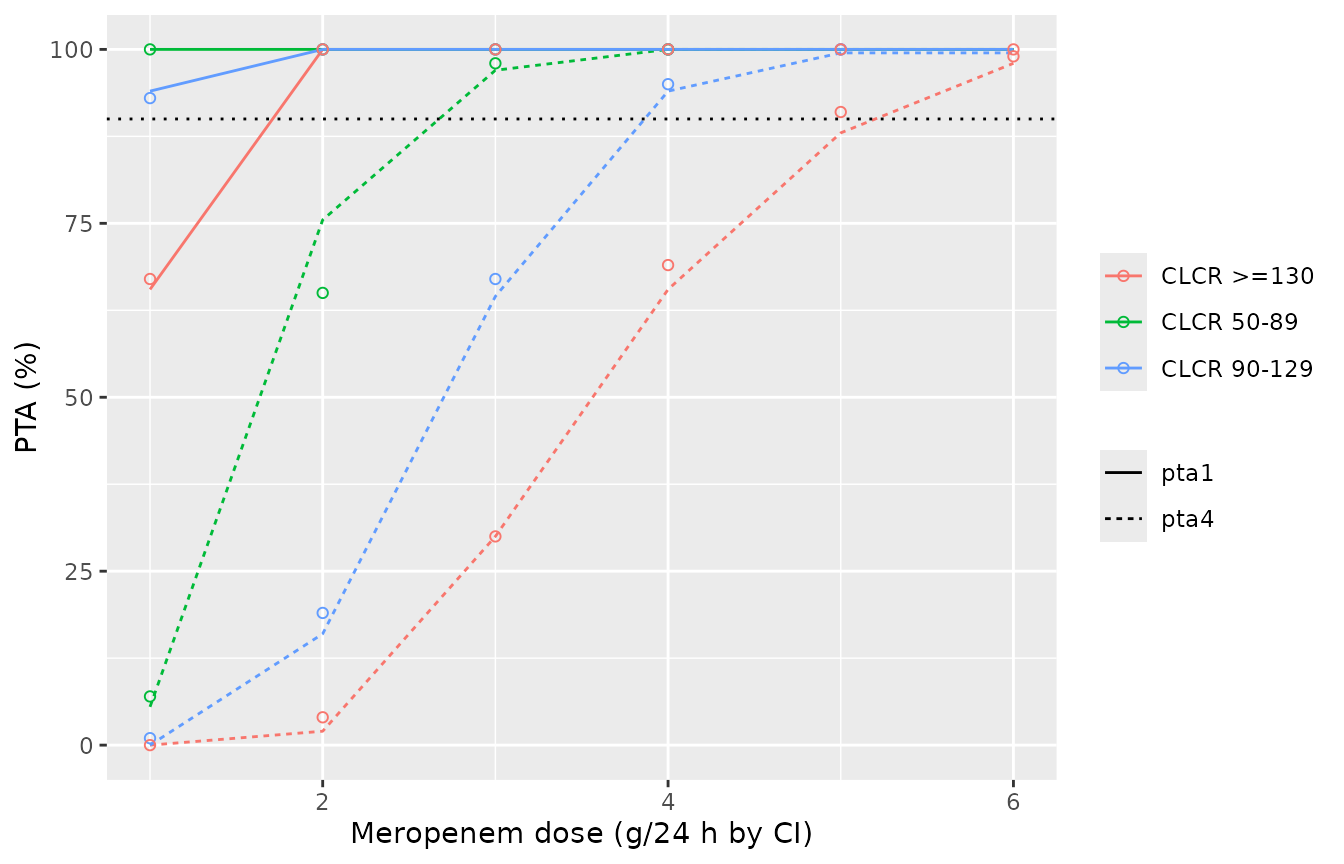
Replicates Figure 4 of Cojutti 2020: PTA of Css/MIC >= 4 (solid) and >= 1 (dashed) at MIC 2 mg/L. Lines are the simulation, points are read from the published figure.
The daily dose at which half of a class reaches Css >= 8 mg/L is the dose at which the class’s median Css equals 8 mg/L, so it depends only on the centre of the clearance distribution and not on which subjects land in the tails. The published crossing is interpolated linearly between the Figure 4 points.
d50_sim <- css |>
  dplyr::filter(!grepl("Study", treatment)) |>
  dplyr::group_by(treatment) |>
  dplyr::summarise(d50_sim = 8 * stats::median(cl) * 24 / 1000)

d50_paper <- pta_paper |>
  dplyr::group_by(treatment) |>
  dplyr::summarise(d50_paper = stats::approx(pta4_paper, daily_g, xout = 50, ties = mean)$y)

d50 <- dplyr::inner_join(d50_sim, d50_paper, by = "treatment") |>
  dplyr::mutate(pct_diff = 100 * (d50_sim / d50_paper - 1))
knitr::kable(d50, digits = 2)| treatment | d50_sim | d50_paper | pct_diff |
|---|---|---|---|
| CLCR 50-89 | 1.61 | 1.74 | -7.45 |
| CLCR 90-129 | 2.63 | 2.65 | -0.56 |
| CLCR >=130 | 3.54 | 3.51 | 0.74 |
PKNCA validation
The paper reports no NCA, only the observed Css distribution of the TDM samples (median 10.5 mg/L at a median regimen of 1 g q8h CI). PKNCA summarises the last 8-h interval of the study-cohort arm, and the average concentration is compared with that observed median.
t_start <- 40
sim_nca <- sim |>
  dplyr::filter(!is.na(Cc), time >= t_start, grepl("Study", treatment)) |>
  dplyr::mutate(time = time - t_start) |>
  dplyr::select(id, time, Cc, treatment)

dose_nca <- sim_nca |>
  dplyr::distinct(id, treatment) |>
  dplyr::mutate(time = 0, amt = dose_mg)

conc_obj <- PKNCA::PKNCAconc(sim_nca, Cc ~ time | treatment + id)
dose_obj <- PKNCA::PKNCAdose(dose_nca, amt ~ time | treatment + id)
intervals <- data.frame(start = 0, end = tau, cav = TRUE, cmax = TRUE, cmin = TRUE, auclast = TRUE)
nca_res <- PKNCA::pk.nca(PKNCA::PKNCAdata(conc_obj, dose_obj, intervals = intervals))
summary(nca_res)
#>  start end                          treatment   N     auclast        cmax
#>      0   8 Study cohort (1 g LD + 1 g q8h CI) 200 76.6 [35.7] 9.55 [35.8]
#>         cmin         cav
#>  9.55 [35.8] 9.57 [35.7]
#>
#> Caption: auclast, cmax, cmin, cav: geometric mean and geometric coefficient of variation; N: number of subjects
reference <- data.frame(treatment = unique(sim_nca$treatment), cav = 10.5)
cmp <- nlmixr2lib::ncaComparisonTable(
  nca_res, reference,
  by = "treatment", params = "cav",
  units = c(cav = "mg/L")
)
knitr::kable(cmp)| NCA parameter | treatment | Reference | Simulated | % diff |
|---|---|---|---|---|
| Cavg (mg/L) | Study cohort (1 g LD + 1 g q8h CI) | 10.5 | 9.47 | -9.8% |
The simulated median Cavg is somewhat below the observed median Css. This is expected rather than a discrepancy: the observed samples came from TDM-adjusted regimens (doses were raised in patients below 8 mg/L), whereas the simulation holds every subject at 1 g q8h.
Assumptions and deviations
- Non-parametric to parametric. Pmetrics NPAG estimates a discrete joint density. It is represented here by log-normal random effects whose variances reproduce the Table 2 CV% (omega^2 = log(CV^2 + 1)), with the Table 2 mean as the typical value. Correlations between support-point parameters are not reported, so the three etas are independent. The mean-over-median choice is supported by both the reported mean clearance and the Figure 4 replication.
-
Random effect on the CRCL slope. NPAG places every
estimated parameter, including the slope theta2, in the joint density,
so theta2 carries its own eta (as in
Downes_2023_vancomycin_full). -
Residual error. Pmetrics’ gamma model gives SD = G
x (C0 + C1 x C); the printed C0 = 0.224, C1 = 0.060 and G = 5 give addSd
= 1.12 mg/L and propSd = 0.30 combined linearly
(
combined1()). - CLCR within Monte Carlo classes. The paper sampled CLCR from normal distributions within each class, but did not print the class means or SDs; uniform draws within the class limits are used, with 170 mL/min/1.73 m^2 as the ARC upper bound (Figure 3).
- Figure 4 values were read from the published plot by the maintainers and are approximate to about +/- 2 percentage points.
- Table 1 / Results inconsistency. The observed Css is printed as “10.5 (8.3-10.2)” mg/L, a median outside its own IQR; the median is used as printed.
-
CRCL uncentred. The model uses the paper’s
uncentred linear form, so
lclis the clearance at CRCL = 0 (non-renal clearance), not at a typical renal function.