Ad26.COV2.S COVID-19 vaccine antibody persistence (Dari 2023)
Source:vignettes/articles/Dari_2023_ad26cov2s.Rmd
Dari_2023_ad26cov2s.RmdModel and source
- Citation: Dari A, Boulton M, Neyens M, Le Gars M, Valenzuela B, Shukarev G, Cardenas V, Ruiz-Guinazu J, Sadoff J, Hoetelmans RMW, Perez Ruixo JJ. Quantifying Antibody Persistence After a Single Dose of COVID-19 Vaccine Ad26.COV2.S in Humans Using a Mechanistic Modeling and Simulation Approach. Clin Pharmacol Ther. 2023;113(2):380. doi:10.1002/cpt.2796.
- Article: https://doi.org/10.1002/cpt.2796 (open access, PMC10107600)
Dari 2023 fit the same six-compartment mechanistic model of the humoral immune response to two antibody read-outs measured after a single 5 x 10^10 viral-particle (vp) dose of Ad26.COV2.S:
-
Dari_2023_ad26cov2s_selisa– spike-protein-binding antibody, S-ELISA (EU/mL), 220 participants. This model was fit first. -
Dari_2023_ad26cov2s_wtvna– neutralizing antibody, wild-type virus neutralization assay (wtVNA, IC50 titer), 82 participants. The systemic parameters (antigen, memory-B-cell and plasma-cell kinetics, and the age effect) were held at the S-ELISA estimates and only the antibody-production parameters, the sex effect and the variability terms were re-estimated.
The two fits are sequential but separate (different datasets, different random effects), so they are packaged as two models. Both are the paper’s “final updated model”, which added the day-169 and day-239 visits and is the model behind every simulation in the paper.
The model (Dari 2023 Eq. 1-6, Figure 1): a K-PD virtual antigen
compartment (antigen) decays at k_ag; antigen
drives memory-B-cell (bcell_memory) production at
kp_ag, which also self-replicates logistically
(kp_m, ceiling n_mem) and differentiates, by a
second-order antigen x memory-B-cell process, into short-lived
(plasma_short) and long-lived (plasma_long)
plasma cells. Plasma cells secrete antibody (kab_s,
kab_l) into serum (antibody), which
distributes to a peripheral compartment (antibody_periph)
and is eliminated (ke_ab). The observation Cc
is the serum antibody level.
mod_s <- readModelDb("Dari_2023_ad26cov2s_selisa")
mod_v <- readModelDb("Dari_2023_ad26cov2s_wtvna")
lloq <- c(selisa = 50.3, wtvna = 58) # Methods, 'Immunogenicity assays'
Population
Healthy SARS-CoV-2-seronegative adults (no prior infection or COVID-19 vaccination) aged 18-55 or >= 65 years from the phase I/IIa COV1001 study (cohorts 1a and 3) and the phase IIa COV2001 study (group 5), who received a single 5 x 10^10 vp dose of Ad26.COV2.S. Participants aged 56-64 years were not included. Samples were drawn on days 1, 15, 29, 57, (64,) 71, 85, 169 and 239.
From Table 1: the S-ELISA analysis set had 220 participants (1,185
titers), median age 52.5 years (range 18-82), 46.8% women, 47.3% aged
>= 60 years, median weight 72.1 kg, 86.4% White non-Hispanic,
enrolled in the United States, Belgium, the Netherlands, Spain and
Germany. The wtVNA set had 82 participants (442 titers), median age 47.5
years (range 18-75), 42.7% women, 42.7% aged >= 60 years, median
weight 72.7 kg, enrolled in Belgium, the Netherlands and Spain. The same
information is in each model’s population metadata.
Source trace
Every value below is a Table 2 entry of Dari 2023 unless stated
otherwise; the in-file comments in
inst/modeldb/specificDrugs/Dari_2023_ad26cov2s_*.R carry
the same trace.
| Parameter | S-ELISA | wtVNA | Source |
|---|---|---|---|
k_ag (1/day) |
0.065 (fixed) | 0.065 (fixed) | Table 2; Balelli 2020 |
kp_ag (cells/antigen unit/day) |
1 (fixed) | 1 (fixed) | Table 2; nonidentifiable, set to 1 |
kp_m, age < 60 y (1/day) |
0.523 | 0.523 (from S-ELISA) | Table 2 |
ke_m (1/day) |
0 (fixed) | 0 (fixed) | Table 2 (0 /year) |
n_mem (cells) |
3.019 x 10^4 (fixed) | 3.019 x 10^4 (fixed) | Table 2; Goel 2021 |
kp_spl = kpS + kpL |
0.691 x 10^-5 | 0.691 x 10^-5 (from S-ELISA) | Table 2 |
r_kp_s_l = kpS/kpL |
2.5/0.011 (fixed) | 2.5/0.011 (fixed) | Table 2; Balelli 2020 |
kp_s, kp_l
|
derived | derived | Table 2 ‘Derived’ rows: kpS = kpSpL/(1 + 0.011/2.5), kpL = kpSpL - kpS |
ke_s (1/day) |
0.578 (fixed) | 0.578 (fixed) | Table 2; Pasin 2019 |
ke_l (1/day) |
16.8 x 10^-4 | 0 (fixed) | Table 2 (final updated model); Supplementary Materials 1.4 |
kab_s |
0.530 | 0.603 | Table 2 |
kab_l, males |
4.43 | 1.86 | Table 2 |
kab_p, kp_ab, ke_ab
(1/day) |
0.2075, 0.2716, 0.0556 (fixed) | same | Table 2; Davda 2014 |
e_age_ge60_kp_m |
-0.441 | -0.441 (from S-ELISA) | Table 2; form kpM * (1 + e * AGE_GE60), Supplementary
Materials 1.7 |
e_sexf_kab_l |
0.671 | 1.10 | Table 2; form kAbL * (1 + e * SEXF)
|
IIV on kp_m (CV) |
78.5% | none | Table 2 (final updated model);
omega^2 = log(1 + CV^2)
|
IIV on kab_s (CV) |
147% | 102% | Table 2 (final updated model) |
IIV on kab_l (CV) |
141% | 104% | Table 2 (final updated model) |
| Residual SD (log10 scale) | 0.117 | 0.191 | Table 2 ‘Proportional error’ (final updated model); see Assumptions |
Antigen dose (amt) |
500 (x 10^8 vp) | 500 (x 10^8 vp) | Not stated; see the next section |
| ODEs | Eq. 1-6 | Eq. 1-6 | Methods, ‘Structural model’ |
Antigen dose scale
The paper gives kp_ag in cells/vp/day and
kp_spl in 1/day/vp, but never states the number entered as
the antigen dose. Entering the nominal 5 x 10^10 vp literally makes
every titer about 10^11. The maintainers therefore solved the
typical-value model (reference subject: man aged < 60 years) for each
power-of-ten unit of the nominal dose and compared it with the observed
median of Figure 2 (digitised by the maintainers to about +/- 0.1
log10).
obs_days <- c(14, 28, 56, 84, 168, 239)
# Figure 2 observed medians (red solid lines), log10 scale, digitised.
fig2_median <- tibble::tribble(
  ~assay,   ~time, ~fig2_log10,
  "selisa",    14, 2.30,
  "selisa",    28, 2.60,
  "selisa",    56, 2.70,
  "selisa",    84, 2.65,
  "selisa",   168, 2.55,
  "selisa",   239, 2.60,
  "wtvna",     14, 2.35,
  "wtvna",     28, 2.50,
  "wtvna",     56, 2.50,
  "wtvna",     84, 2.40,
  "wtvna",    168, 2.40,
  "wtvna",    239, 2.40
)

typical_profile <- function(mod, amt) {
  ev <- rxode2::et(amt = amt, cmt = "antigen") |>
    rxode2::et(obs_days, cmt = "antibody") |>
    as.data.frame() |>
    dplyr::mutate(SEXF = 0, AGE_GE60 = 0)
  sim <- rxode2::rxSolve(rxode2::zeroRe(mod), ev, returnType = "data.frame")
  sim[, c("time", "Cc")]
}

dose_units <- c(
  "1e9 vp (amt = 50)" = 50,
  "1e8 vp (amt = 500)" = 500,
  "1e7 vp (amt = 5000)" = 5000,
  "vp (amt = 5e10)" = 5e10
)
scale_check <- dplyr::bind_rows(lapply(names(dose_units), function(u) {
  dplyr::bind_rows(
    typical_profile(mod_s, dose_units[[u]]) |> dplyr::mutate(assay = "selisa"),
    typical_profile(mod_v, dose_units[[u]]) |> dplyr::mutate(assay = "wtvna")
  ) |>
    dplyr::mutate(dose_unit = u)
})) |>
  dplyr::mutate(log10_Cc = log10(Cc)) |>
  dplyr::left_join(fig2_median, by = c("assay", "time"))
#> ℹ parameter labels from comments will be replaced by 'label()'
#> ℹ omega/sigma items treated as zero: 'etalkp_m', 'etalkab_s', 'etalkab_l'
#> ℹ parameter labels from comments will be replaced by 'label()'
#> ℹ omega/sigma items treated as zero: 'etalkab_s', 'etalkab_l'
#> ℹ parameter labels from comments will be replaced by 'label()'
#> ℹ omega/sigma items treated as zero: 'etalkp_m', 'etalkab_s', 'etalkab_l'
#> ℹ parameter labels from comments will be replaced by 'label()'
#> ℹ omega/sigma items treated as zero: 'etalkab_s', 'etalkab_l'
#> ℹ parameter labels from comments will be replaced by 'label()'
#> ℹ omega/sigma items treated as zero: 'etalkp_m', 'etalkab_s', 'etalkab_l'
#> ℹ parameter labels from comments will be replaced by 'label()'
#> ℹ omega/sigma items treated as zero: 'etalkab_s', 'etalkab_l'
#> ℹ parameter labels from comments will be replaced by 'label()'
#> ℹ omega/sigma items treated as zero: 'etalkp_m', 'etalkab_s', 'etalkab_l'
#> ℹ parameter labels from comments will be replaced by 'label()'
#> ℹ omega/sigma items treated as zero: 'etalkab_s', 'etalkab_l'

scale_check |>
  dplyr::select(dose_unit, assay, time, log10_Cc) |>
  tidyr::pivot_wider(names_from = time, values_from = log10_Cc) |>
knitr::kable(digits = 2, caption = "Typical-value log10 titer by day after vaccination, for each candidate dose unit.")| dose_unit | assay | 14 | 28 | 56 | 84 | 168 | 239 |
|---|---|---|---|---|---|---|---|
| 1e9 vp (amt = 50) | selisa | 0.87 | 1.40 | 1.48 | 1.45 | 1.37 | 1.31 |
| 1e9 vp (amt = 50) | wtvna | 0.90 | 1.39 | 1.37 | 1.25 | 1.09 | 1.07 |
| 1e8 vp (amt = 500) | selisa | 2.30 | 2.56 | 2.61 | 2.57 | 2.49 | 2.43 |
| 1e8 vp (amt = 500) | wtvna | 2.32 | 2.54 | 2.48 | 2.36 | 2.21 | 2.19 |
| 1e7 vp (amt = 5000) | selisa | 3.59 | 3.74 | 3.75 | 3.71 | 3.63 | 3.57 |
| 1e7 vp (amt = 5000) | wtvna | 3.60 | 3.70 | 3.61 | 3.49 | 3.35 | 3.34 |
| vp (amt = 5e10) | selisa | 11.34 | 11.46 | 11.46 | 11.43 | 11.34 | 11.29 |
| vp (amt = 5e10) | wtvna | 11.35 | 11.41 | 11.31 | 11.20 | 11.07 | 11.05 |
scale_fit <- scale_check |>
  dplyr::group_by(dose_unit, assay) |>
  dplyr::summarise(
    mean_abs_log10_diff = mean(abs(log10_Cc - fig2_log10)),
    .groups = "drop"
  )
knitr::kable(scale_fit, digits = 2, caption = "Mean absolute difference from the Figure 2 observed median (log10 units).")| dose_unit | assay | mean_abs_log10_diff |
|---|---|---|
| 1e7 vp (amt = 5000) | selisa | 1.10 |
| 1e7 vp (amt = 5000) | wtvna | 1.09 |
| 1e8 vp (amt = 500) | selisa | 0.07 |
| 1e8 vp (amt = 500) | wtvna | 0.09 |
| 1e9 vp (amt = 50) | selisa | 1.25 |
| 1e9 vp (amt = 50) | wtvna | 1.25 |
| vp (amt = 5e10) | selisa | 8.82 |
| vp (amt = 5e10) | wtvna | 8.81 |
# Deterministic typical-value solves, so the bounds can be tight. Only the
# 10^8-vp unit lands within a few tenths of a log10 of the observed median;
# the neighbouring units miss by more than one log10 for both assays.
fit_of <- function(unit, a) {
  scale_fit$mean_abs_log10_diff[scale_fit$dose_unit == unit & scale_fit$assay == a]
}
stopifnot(
  fit_of("1e8 vp (amt = 500)", "selisa") < 0.2,
  fit_of("1e8 vp (amt = 500)", "wtvna") < 0.2,
  fit_of("1e9 vp (amt = 50)", "selisa") > 1,
  fit_of("1e7 vp (amt = 5000)", "selisa") > 0.8,
  fit_of("1e9 vp (amt = 50)", "wtvna") > 1,
  fit_of("1e7 vp (amt = 5000)", "wtvna") > 0.8
)
The vaccine dose is therefore entered as amt = 500 in
units of 10^8 vp. The persistence projections further down (Table 3, S1
and S2) are an independent check of the same choice: they depend on the
dose scale through the fraction of participants whose titers sit near
the LLOQ.
Virtual cohorts
# One dosing record per subject plus observation records on the serum
# antibody state; each subject carries its own sex and age indicators.
make_events <- function(SEXF, AGE_GE60, obs_times, id_offset = 0L) {
  n <- length(SEXF)
  ids <- id_offset + seq_len(n)
  covs <- data.frame(id = ids, SEXF = SEXF, AGE_GE60 = AGE_GE60)
  dose <- data.frame(id = ids, time = 0, evid = 1L, amt = 500, cmt = "antigen")
  obs <- expand.grid(time = obs_times, id = ids)
  obs$evid <- 0L
  obs$amt <- 0
  obs$cmt <- "antibody"
  dplyr::bind_rows(dose, obs[, names(dose)]) |>
    dplyr::left_join(covs, by = "id") |>
    dplyr::arrange(id, time, dplyr::desc(evid))
}
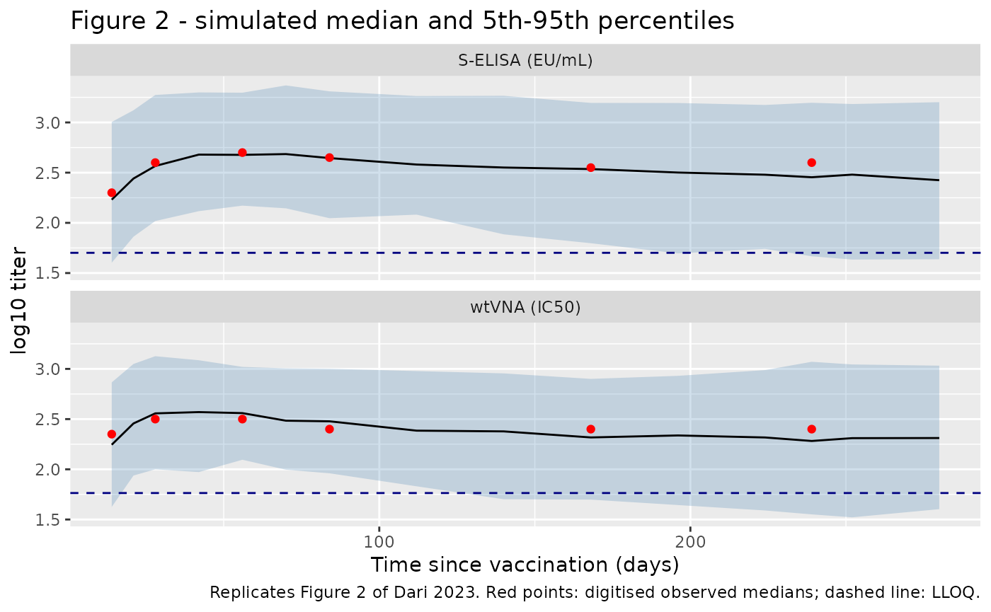
Figure 2: visual predictive check
Each assay’s cohort has 200 participants with the Table 1 proportions
of women and of participants aged >= 60 years. sim
includes the residual error, as the paper’s VPC does.
rxode2::rxSetSeed(2023)
set.seed(2023)
vpc_days <- c(14, 21, 28, 42, 56, 70, 84, 112, 140, 168, 196, 224, 239, 252, 280)
n_vpc <- 200
ev_s <- make_events(
  SEXF = sample(rep(0:1, c(n_vpc - round(0.468 * n_vpc), round(0.468 * n_vpc)))),
  AGE_GE60 = sample(rep(0:1, c(n_vpc - round(0.473 * n_vpc), round(0.473 * n_vpc)))),
  obs_times = vpc_days
)
ev_v <- make_events(
  SEXF = sample(rep(0:1, c(n_vpc - round(0.427 * n_vpc), round(0.427 * n_vpc)))),
  AGE_GE60 = sample(rep(0:1, c(n_vpc - round(0.427 * n_vpc), round(0.427 * n_vpc)))),
  obs_times = vpc_days
)
sim_vpc <- dplyr::bind_rows(
  rxode2::rxSolve(mod_s, ev_s, returnType = "data.frame") |> dplyr::mutate(assay = "selisa"),
  rxode2::rxSolve(mod_v, ev_v, returnType = "data.frame") |> dplyr::mutate(assay = "wtvna")
)
#> ℹ parameter labels from comments will be replaced by 'label()'
#> ℹ parameter labels from comments will be replaced by 'label()'

vpc <- sim_vpc |>
  dplyr::group_by(assay, time) |>
  dplyr::summarise(
    q05 = quantile(log10(sim), 0.05),
    q50 = quantile(log10(sim), 0.50),
    q95 = quantile(log10(sim), 0.95),
    .groups = "drop"
  )

ggplot(vpc, aes(time, q50)) +
  geom_ribbon(aes(ymin = q05, ymax = q95), fill = "steelblue", alpha = 0.25) +
  geom_line() +
  geom_point(data = fig2_median, aes(time, fig2_log10), colour = "red") +
  geom_hline(
    data = data.frame(assay = names(lloq), y = log10(lloq)),
    aes(yintercept = y), linetype = "dashed", colour = "navy"
  ) +
  facet_wrap(~assay, ncol = 1, labeller = as_labeller(c(selisa = "S-ELISA (EU/mL)", wtvna = "wtVNA (IC50)"))) +
  labs(
    x = "Time since vaccination (days)", y = "log10 titer",
    title = "Figure 2 - simulated median and 5th-95th percentiles",
    caption = "Replicates Figure 2 of Dari 2023. Red points: digitised observed medians; dashed line: LLOQ."
  )
vpc_check <- vpc |>
  dplyr::inner_join(fig2_median, by = c("assay", "time")) |>
  dplyr::mutate(diff = q50 - fig2_log10)
knitr::kable(vpc_check, digits = 2, caption = "Simulated vs digitised observed median (log10).")| assay | time | q05 | q50 | q95 | fig2_log10 | diff |
|---|---|---|---|---|---|---|
| selisa | 14 | 1.60 | 2.23 | 3.00 | 2.30 | -0.07 |
| selisa | 28 | 2.02 | 2.57 | 3.27 | 2.60 | -0.03 |
| selisa | 56 | 2.17 | 2.68 | 3.30 | 2.70 | -0.02 |
| selisa | 84 | 2.05 | 2.65 | 3.31 | 2.65 | 0.00 |
| selisa | 168 | 1.80 | 2.54 | 3.19 | 2.55 | -0.01 |
| selisa | 239 | 1.67 | 2.45 | 3.20 | 2.60 | -0.15 |
| wtvna | 14 | 1.62 | 2.24 | 2.87 | 2.35 | -0.11 |
| wtvna | 28 | 2.00 | 2.56 | 3.13 | 2.50 | 0.06 |
| wtvna | 56 | 2.09 | 2.56 | 3.02 | 2.50 | 0.06 |
| wtvna | 84 | 1.96 | 2.48 | 3.00 | 2.40 | 0.08 |
| wtvna | 168 | 1.70 | 2.32 | 2.90 | 2.40 | -0.08 |
| wtvna | 239 | 1.55 | 2.28 | 3.07 | 2.40 | -0.12 |
# The simulated median has a sampling SD of about 0.05 log10 at n = 200. A
# mis-transcribed production rate, dose or covariate shifts it by > 0.3.
stopifnot(
  abs(median(vpc_check$diff[vpc_check$assay == "selisa"])) < 0.2,
  abs(median(vpc_check$diff[vpc_check$assay == "wtvna"])) < 0.2,
  quantile(abs(vpc_check$diff), 0.9) < 0.3
)
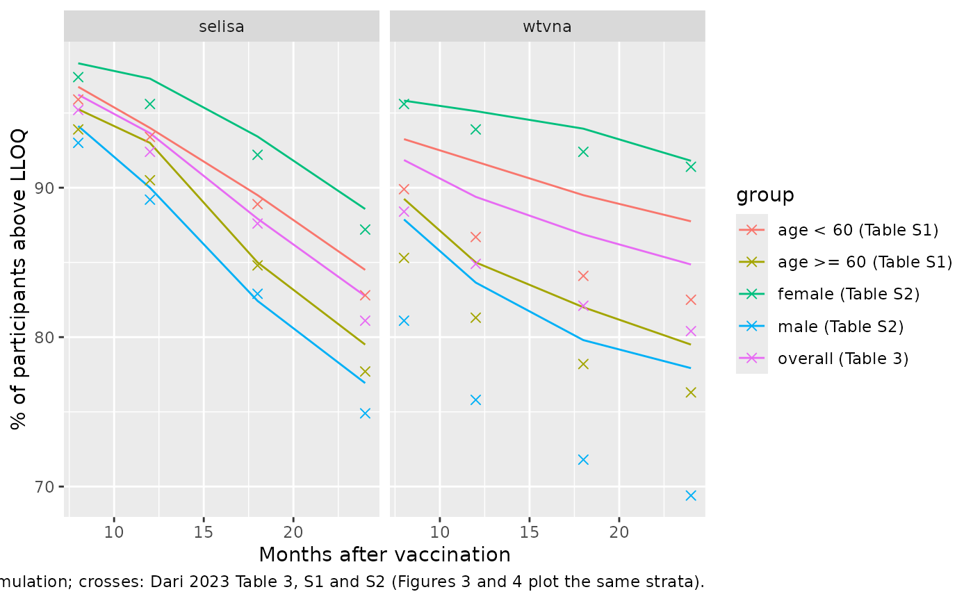
Tables 3, S1 and S2: persistence above the LLOQ
The paper defines individual persistence as the time from vaccination until the last titer above the LLOQ before two consecutive monthly titers below it, and reports the share of participants still persisting at 8, 12, 18 and 24 months. The simulation below follows that rule on monthly simulated observations (including residual error), with 200 participants in each sex x age stratum.
rxode2::rxSetSeed(3)
months <- 1:24
strata <- expand.grid(SEXF = 0:1, AGE_GE60 = 0:1)
n_stratum <- 200
ev_p <- make_events(
  SEXF = rep(strata$SEXF, each = n_stratum),
  AGE_GE60 = rep(strata$AGE_GE60, each = n_stratum),
  obs_times = months * 30.4375
)
stopifnot(!anyDuplicated(ev_p[, c("id", "time", "evid")]))

persistence_months <- function(below) {
  # First month m with titers below the LLOQ at both m and m + 1; persistence
  # ends at the month before it. Never two in a row: persists beyond 24.
  k <- which(below[-length(below)] & below[-1])
  if (length(k) == 0) Inf else k[1] - 1
}

pers <- dplyr::bind_rows(
  rxode2::rxSolve(mod_s, ev_p, returnType = "data.frame", keep = c("SEXF", "AGE_GE60")) |>
    dplyr::mutate(assay = "selisa"),
  rxode2::rxSolve(mod_v, ev_p, returnType = "data.frame", keep = c("SEXF", "AGE_GE60")) |>
    dplyr::mutate(assay = "wtvna")
) |>
  dplyr::arrange(assay, id, time) |>
  dplyr::group_by(assay, id, SEXF, AGE_GE60) |>
  dplyr::summarise(
    persist = persistence_months(sim < lloq[[dplyr::first(assay)]]),
    .groups = "drop"
  )

by_stratum <- tidyr::expand_grid(pers, month = c(8, 12, 18, 24)) |>
  dplyr::group_by(assay, SEXF, AGE_GE60, month) |>
  dplyr::summarise(pct = 100 * mean(persist >= month), .groups = "drop")
The age strata of Table S1 have a 1:1 sex ratio, as in the paper’s simulation. The paper sampled age from the phase III COV3001 age distribution for Table 3 and Table S2; the share of participants >= 60 years implied by Table 3 and Table S1 is about 0.35 (for example S-ELISA at 8 months: (95.9 - 95.2) / (95.9 - 93.9) = 0.35), which is used to weight the age strata.
w60 <- 0.35
sim_tab <- dplyr::bind_rows(
  by_stratum |>
    dplyr::group_by(assay, month, AGE_GE60) |>
    dplyr::summarise(pct = mean(pct), .groups = "drop") |>
    dplyr::mutate(group = ifelse(AGE_GE60 == 1, "age >= 60 (Table S1)", "age < 60 (Table S1)")),
  by_stratum |>
    dplyr::group_by(assay, month, SEXF) |>
    dplyr::summarise(pct = sum(pct * ifelse(AGE_GE60 == 1, w60, 1 - w60)), .groups = "drop") |>
    dplyr::mutate(group = ifelse(SEXF == 1, "female (Table S2)", "male (Table S2)")),
  by_stratum |>
    dplyr::group_by(assay, month) |>
    dplyr::summarise(pct = sum(pct * 0.5 * ifelse(AGE_GE60 == 1, w60, 1 - w60)), .groups = "drop") |>
    dplyr::mutate(group = "overall (Table 3)")
) |>
  dplyr::select(assay, group, month, pct)

# Predicted % above the LLOQ, Dari 2023 Table 3, Table S1 and Table S2.
paper_tab <- tibble::tribble(
  ~group, ~month, ~selisa, ~wtvna,
  "overall (Table 3)", 8, 95.2, 88.4,
  "overall (Table 3)", 12, 92.4, 84.9,
  "overall (Table 3)", 18, 87.6, 82.1,
  "overall (Table 3)", 24, 81.1, 80.4,
  "age < 60 (Table S1)", 8, 95.9, 89.9,
  "age < 60 (Table S1)", 12, 93.4, 86.7,
  "age < 60 (Table S1)", 18, 88.9, 84.1,
  "age < 60 (Table S1)", 24, 82.8, 82.5,
  "age >= 60 (Table S1)", 8, 93.9, 85.3,
  "age >= 60 (Table S1)", 12, 90.5, 81.3,
  "age >= 60 (Table S1)", 18, 84.8, 78.2,
  "age >= 60 (Table S1)", 24, 77.7, 76.3,
  "male (Table S2)", 8, 93.0, 81.1,
  "male (Table S2)", 12, 89.2, 75.8,
  "male (Table S2)", 18, 82.9, 71.8,
  "male (Table S2)", 24, 74.9, 69.4,
  "female (Table S2)", 8, 97.4, 95.6,
  "female (Table S2)", 12, 95.6, 93.9,
  "female (Table S2)", 18, 92.2, 92.4,
  "female (Table S2)", 24, 87.2, 91.4
) |>
  tidyr::pivot_longer(c(selisa, wtvna), names_to = "assay", values_to = "paper_pct")

persist_cmp <- sim_tab |>
  dplyr::inner_join(paper_tab, by = c("assay", "group", "month")) |>
  dplyr::mutate(diff = pct - paper_pct)
stopifnot(nrow(persist_cmp) == nrow(paper_tab))

persist_cmp |>
  dplyr::arrange(assay, group, month) |>
  dplyr::rename(
    "Assay" = assay, "Group" = group, "Month" = month,
    "Simulated %" = pct, "Paper %" = paper_pct, "Difference" = diff
  ) |>
knitr::kable(digits = 1, caption = "Predicted percentage of participants with persisting titers above the LLOQ.")| Assay | Group | Month | Simulated % | Paper % | Difference |
|---|---|---|---|---|---|
| selisa | age < 60 (Table S1) | 8 | 96.8 | 95.9 | 0.8 |
| selisa | age < 60 (Table S1) | 12 | 94.0 | 93.4 | 0.6 |
| selisa | age < 60 (Table S1) | 18 | 89.5 | 88.9 | 0.6 |
| selisa | age < 60 (Table S1) | 24 | 84.5 | 82.8 | 1.7 |
| selisa | age >= 60 (Table S1) | 8 | 95.2 | 93.9 | 1.3 |
| selisa | age >= 60 (Table S1) | 12 | 93.0 | 90.5 | 2.5 |
| selisa | age >= 60 (Table S1) | 18 | 85.0 | 84.8 | 0.2 |
| selisa | age >= 60 (Table S1) | 24 | 79.5 | 77.7 | 1.8 |
| selisa | female (Table S2) | 8 | 98.3 | 97.4 | 0.9 |
| selisa | female (Table S2) | 12 | 97.3 | 95.6 | 1.7 |
| selisa | female (Table S2) | 18 | 93.4 | 92.2 | 1.2 |
| selisa | female (Table S2) | 24 | 88.6 | 87.2 | 1.4 |
| selisa | male (Table S2) | 8 | 94.1 | 93.0 | 1.1 |
| selisa | male (Table S2) | 12 | 90.0 | 89.2 | 0.8 |
| selisa | male (Table S2) | 18 | 82.4 | 82.9 | -0.5 |
| selisa | male (Table S2) | 24 | 76.9 | 74.9 | 2.0 |
| selisa | overall (Table 3) | 8 | 96.2 | 95.2 | 1.0 |
| selisa | overall (Table 3) | 12 | 93.6 | 92.4 | 1.2 |
| selisa | overall (Table 3) | 18 | 87.9 | 87.6 | 0.3 |
| selisa | overall (Table 3) | 24 | 82.8 | 81.1 | 1.7 |
| wtvna | age < 60 (Table S1) | 8 | 93.2 | 89.9 | 3.3 |
| wtvna | age < 60 (Table S1) | 12 | 91.8 | 86.7 | 5.0 |
| wtvna | age < 60 (Table S1) | 18 | 89.5 | 84.1 | 5.4 |
| wtvna | age < 60 (Table S1) | 24 | 87.8 | 82.5 | 5.2 |
| wtvna | age >= 60 (Table S1) | 8 | 89.2 | 85.3 | 4.0 |
| wtvna | age >= 60 (Table S1) | 12 | 85.0 | 81.3 | 3.7 |
| wtvna | age >= 60 (Table S1) | 18 | 82.0 | 78.2 | 3.8 |
| wtvna | age >= 60 (Table S1) | 24 | 79.5 | 76.3 | 3.2 |
| wtvna | female (Table S2) | 8 | 95.8 | 95.6 | 0.2 |
| wtvna | female (Table S2) | 12 | 95.1 | 93.9 | 1.2 |
| wtvna | female (Table S2) | 18 | 93.9 | 92.4 | 1.5 |
| wtvna | female (Table S2) | 24 | 91.8 | 91.4 | 0.4 |
| wtvna | male (Table S2) | 8 | 87.9 | 81.1 | 6.8 |
| wtvna | male (Table S2) | 12 | 83.7 | 75.8 | 7.9 |
| wtvna | male (Table S2) | 18 | 79.8 | 71.8 | 8.0 |
| wtvna | male (Table S2) | 24 | 77.9 | 69.4 | 8.5 |
| wtvna | overall (Table 3) | 8 | 91.8 | 88.4 | 3.4 |
| wtvna | overall (Table 3) | 12 | 89.4 | 84.9 | 4.5 |
| wtvna | overall (Table 3) | 18 | 86.9 | 82.1 | 4.8 |
| wtvna | overall (Table 3) | 24 | 84.9 | 80.4 | 4.5 |
ggplot(persist_cmp, aes(month, pct, colour = group)) +
  geom_line() +
  geom_point(aes(y = paper_pct), shape = 4, size = 2) +
  facet_wrap(~assay) +
  labs(
    x = "Months after vaccination", y = "% of participants above LLOQ",
    caption = "Lines: simulation; crosses: Dari 2023 Table 3, S1 and S2 (Figures 3 and 4 plot the same strata)."
  )
# With 200 participants per stratum a single cell has a sampling SD of 2-3
# percentage points, and the cells of one assay move together because they
# share subjects. The wtVNA cells also sit about 3 points above the paper
# even in a 4,000-subject run (see the text below). One draw gave a median
# difference of 1.7 and a 90th percentile of about 6. A dose unit one power
# of ten off moves every cell by tens of points.
stopifnot(
  abs(median(persist_cmp$diff)) < 5,
  quantile(abs(persist_cmp$diff), 0.9) < 10
)
# The sex contrast for wtVNA at 24 months is the paper's headline (69.4% men
# vs 91.4% women); its size, not just its sign, is checked.
wt24 <- sim_tab |> dplyr::filter(assay == "wtvna", month == 24)
stopifnot(
  wt24$pct[wt24$group == "female (Table S2)"] - wt24$pct[wt24$group == "male (Table S2)"] > 10
)
The S-ELISA projections agree with Tables 3, S1 and S2 to within a few percentage points. The wtVNA projections run high, by about 3 points in a 4,000-subject run and most in men, where more titers sit close to the LLOQ. The likely cause is that the paper also sampled parameter uncertainty, which widens the titer distribution and moves more participants below the LLOQ; this vignette simulates the point estimates only.
PKNCA: peak antibody response
The paper reports no non-compartmental summaries, so this block only records the simulated individual peak titer and its timing (no residual error) for the Figure 2 cohorts, by assay and sex.
nca_in <- sim_vpc |>
  dplyr::filter(!is.na(Cc)) |>
  dplyr::mutate(group = paste(assay, ifelse(SEXF == 1, "female", "male"))) |>
  dplyr::select(id, time, Cc, group)
nca_in <- dplyr::bind_rows(
  nca_in,
  nca_in |> dplyr::distinct(id, group) |> dplyr::mutate(time = 0, Cc = 0)
) |>
  dplyr::arrange(group, id, time)
stopifnot(all(nca_in$time[!duplicated(nca_in[, c("group", "id")])] == 0))

dose_in <- nca_in |>
  dplyr::distinct(id, group) |>
  dplyr::mutate(time = 0, amt = 500)

nca_res <- PKNCA::pk.nca(PKNCA::PKNCAdata(
  PKNCA::PKNCAconc(nca_in, Cc ~ time | group + id),
  PKNCA::PKNCAdose(dose_in, amt ~ time | group + id),
  intervals = data.frame(start = 0, end = 280, cmax = TRUE, tmax = TRUE)
))
nca_sum <- as.data.frame(nca_res) |>
  dplyr::filter(PPTESTCD %in% c("cmax", "tmax")) |>
  dplyr::group_by(group, PPTESTCD) |>
  dplyr::summarise(median = median(PPORRES), .groups = "drop") |>
  tidyr::pivot_wider(names_from = PPTESTCD, values_from = median)
nca_sum |>
  dplyr::rename("Assay and sex" = group, "Median Cmax (titer)" = cmax, "Median Tmax (day)" = tmax) |>
knitr::kable(digits = 0, caption = "Simulated peak antibody response.")| Assay and sex | Median Cmax (titer) | Median Tmax (day) |
|---|---|---|
| selisa female | 718 | 84 |
| selisa male | 479 | 56 |
| wtvna female | 503 | 42 |
| wtvna male | 371 | 42 |
The median peak falls on the plateau that the Figure 2 medians show between days 28 and 84, and women peak higher than men because of the sex effect on long-lived-plasma-cell antibody production.
Assumptions and deviations
-
Antigen dose scale (not stated in the paper). The
vaccine dose enters the K-PD antigen compartment as
amt = 500, i.e. the 5 x 10^10 vp dose in units of 10^8 vp. The paper giveskp_agandkp_splper vp but never the amount entered; the literal 5 x 10^10 gives titers near 10^11. The maintainers compared each power-of-ten unit of the nominal dose and kept the only one that reproduces both the Figure 2 medians and the Table 3 / S1 / S2 persistence (see above). No continuous fitting was done. -
Residual error scale. Supplementary Materials 1.6
states an additive error on log10 titers; Table 2 reports it as
“Proportional error” 11.7 (S-ELISA) and 19.1 (wtVNA) in a column headed
CV%. The maintainers read these as log10-scale SDs x 100 (0.117 and
0.191) and encode them as
lnorm()SDs on the natural-log scale (0.2694 and 0.4398). Reading them as CVs on the original scale (natural-log SD 0.117 and 0.189) leaves the simulated wtVNA persistence almost flat after month 8 (about 89% at 24 months), against 80.4% in Table 3; the log10 reading gives 83-85%. -
Final model vs final updated model. Only the final
updated model (day-239 data,
ke_lestimated for S-ELISA, IIV and residual error re-estimated) is packaged. The day-85 final model shares the same structural estimates withke_l = 0; its IIV and residual-error values are recorded in the model-file comments. - Persistence simulation. The paper simulated 250,000 participants with parameter uncertainty and drew age from the COV3001 distribution; this vignette uses 200 participants per sex x age stratum, no parameter uncertainty, and weights the age strata 0.65 / 0.35, the split implied by Table 3 and Table S1.
-
Observation name. The serum antibody output is
named
Cc, as for the anti-RBD IgG output ofDasti_2025_mrna1273_qsp, although it is an antibody response and not a concentration of the administered vaccine. -
Screened covariates. Body weight, race and country
were screened and not retained; they appear in
covariatesDataExcluded(body weight) and in the model notes. - No erratum or correction notice for Dari 2023 was found in Europe PMC (search and citation list) as of 2026-10-26.