Meropenem in-bottle degradation and PK (Tien 2024)
Source:vignettes/articles/Tien_2024_meropenem.Rmd
Tien_2024_meropenem.RmdModel and source
- Citation: Tien NTN, Binh VN, Ha PTT, Lan DTN, Cho YS, Long NP, Shin JG, Anh NH, Quan TA, Tuan DN, Tiep NK, Thach PT, Anh NH, Hoa VD. Optimization of meropenem continuous infusion based on Monte Carlo simulation integrating with degradation study. PLoS One. 2024;19(12):e0313764. doi:10.1371/journal.pone.0313764. Stability model: Methods Eq. 1, Table 2 and the full-precision lmer output in S3 File; coupled PK/degradation equations: Methods ‘Simulation procedure’ and S4 File. PK parameters as recoded in S4 File from Ehmann L et al. Int J Antimicrob Agents. 2019;54(3):309-317, doi:10.1016/j.ijantimicag.2019.06.016.
- Description: Meropenem in-bottle degradation coupled to a two-compartment population PK model in critically ill adults without CRRT (Tien 2024). The infusion solution is an ODE state (infusion_container) dosed as a bolus when the bottle is hung; intact drug degrades by first-order kinetics and is pumped into central at constant volume rate over TINF, so the delivery rate is Dose * exp(-kdeg * t) / TINF. kdeg comes from a linear mixed-effects fit to in-vitro stability data (7 generic brands, 1 or 2 g/48 mL in saline, 25/30/37 degC, 0-8 h) with categorical solution-temperature and solution-strength effects and correlated random intercept and slope per bottle series; the in-vitro fraction remaining is a second output with additive error on log(C/C0). The PK layer is the Ehmann 2019 ICU model as recoded by Tien: CL linear in Cockcroft-Gault creatinine clearance (centred 80.8 mL/min) up to an estimated hinge at 154 mL/min, power weight effect on Vc and linear albumin effect on Vp, with IIV on CL, Vc and Vp and one occasion of IOV on CL.
- Article: https://doi.org/10.1371/journal.pone.0313764 (open
access, with the stability data, the
lmercode and the RxODE simulation code as S2-S4 Files)
Tien et al. measured how fast meropenem degrades in a prepared infusion bottle, then fed that loss into a published ICU population PK model to ask whether the loss matters for target attainment during prolonged and continuous infusion. The packaged model keeps both layers in one file because they are coupled: the bottle is an ODE state whose intact drug decays while the pump delivers it to the central compartment.
Population
Stability study (in vitro). Seven generic meropenem brands were reconstituted in 0.9% sodium chloride at 1 g/48 mL and 2 g/48 mL, held at 25, 30 and 37 degC, and assayed by HPLC hourly for 8 h: 42 bottle series and 365 retained observations (Results; S2 and S3 Files). Brand did not improve the fit (Table 1, Model 4, p = 0.14), so the final model has temperature and strength effects only.
PK layer. Tien used the Ehmann 2019 model for critically ill adults with severe infections who were not on continuous renal replacement therapy (48 patients, 1376 samples; creatinine clearance median 70.8 mL/min, 5th-95th percentiles 34.8-160 mL/min; Methods). The typical patient of the deterministic simulations has CRCL 80.8 mL/min, weight 70 kg and albumin 2.8 g/dL.
str(rxode2::rxode(readModelDb("Tien_2024_meropenem"))$population)
#> List of 9
#>  $ species       : chr "human (PK layer) + in vitro (infusion-solution stability)"
#>  $ n_subjects    : num 48
#>  $ n_studies     : num 1
#>  $ disease_state : chr "Critically ill adults with severe infections, not on continuous renal replacement therapy (Ehmann 2019 PK cohort)."
#>  $ renal_function: chr "Cockcroft-Gault creatinine clearance median 70.8 mL/min, 5th-95th percentiles 34.8-160 mL/min (Methods, citing Ehmann 2019)."
#>  $ n_observations: chr "1376 plasma samples (PK); 365 in-vitro stability observations"
#>  $ in_vitro      : chr "Seven meropenem generic brands reconstituted in 0.9% sodium chloride at 1 g/48 mL and 2 g/48 mL, held at 25, 30"| __truncated__
#>  $ regions       : chr "Vietnam (stability study); the PK cohort's region is not stated in Tien 2024"
#>  $ notes         : chr "Typical patient of the deterministic simulations: CRCL 80.8 mL/min, WT 70 kg, albumin 2.8 g/dL. Monte Carlo sim"| __truncated__
Source trace
| Model element | Value | Source |
|---|---|---|
Stability model
log(C/C0) = mu + theta - (b0 + b1*T + b2*Cinfu + eta)*t + eps
|
– | Methods Eq. 1; S3 File section 1 |
infusion_log_intercept (mu) |
-0.0002568 | S3 File summary(fit3); Table 2 (-0.0003) |
kdeg (b0, 25 degC, 1 g/48 mL) |
0.0086083 1/h | S3 File; Table 2 (0.0086) |
e_infusion_temp_30c_kdeg |
0.0044789 1/h | S3 File; Table 2 (0.0045) |
e_infusion_temp_37c_kdeg |
0.0185050 1/h | S3 File; Table 2 (0.0185) |
e_form_meropenem_soln2g48ml_kdeg |
0.0041512 1/h | S3 File; Table 2 (0.0042) |
| Random intercept / slope variances, correlation | 4.119e-05, 2.149e-06, 0.94 | S3 File; Table 2 (omega1 0.0064, omega2 0.0015 as SD) |
expSd_infusion_fraction_remaining (sigma) |
0.010127 | S3 File; Table 2 (0.0101) |
Bottle input Dose * exp(-kdeg * t) / Tinf for
t <= Tinf
|
– | Methods ‘Simulation procedure’ equations; Fig 1; S4 File
Depot/duration
|
| Two-compartment ODEs | – | Methods ‘Simulation procedure’ equations; S4 File
@dynamics
|
lcl |
log(9.25) L/h | S4 File tvCL (RSE 4.6%) |
lvc |
log(7.89) L | S4 File tvVc (RSE 11.9%) |
lq |
log(28.4) L/h | S4 File tvQ (RSE 16.1%) |
lvp |
log(16.1) L | S4 File tvVp (RSE 7.4%) |
e_crcl_cl, centred 80.8 mL/min |
0.00977 | S4 File CLCR_CL, @pre block |
lcrcl_hinge |
log(154) mL/min | S4 File CLCR_INF (RSE 6.9%) |
e_wt_vc, reference 70 kg |
0.945 | S4 File WT_Vc
|
e_alb_vp, centred 2.8 g/dL |
-0.202 | S4 File ALB_Vp
|
| IIV CL, Vc, Vp | 27.1, 31.5, 16.9 %CV | Methods; S4 File Omega
|
| IOV CL | 12.5 %CV | Methods; S4 File Omega
|
propSd (Cc) |
fixed(0) | not reported (see Assumptions) |
Simulation helpers
Dosing follows S4 File: a 500 mg loading dose over 30 min, then the
maintenance bottles from 0.5 h. A degradation arm hangs each
bottle as a bolus into infusion_container and sets
TINF to that bottle’s infusion length; a
no-degradation arm gives the same doses as zero-order infusions
straight into central, which is the paper’s reference
model.
mod <- readModelDb("Tien_2024_meropenem")

regimens <- tibble::tribble(
  ~regimen,     ~interval, ~tinf, ~dose,
  "EI 3 h q8h",         8,     3,  1000,
  "CI 3 h",             3,     3,   375,
  "CI 6 h",             6,     6,   750,
  "CI 8 h",             8,     8,  1000
)

conditions <- tibble::tribble(
  ~condition,               ~degrade, ~temp, ~strength,
  "No degradation",         FALSE,    25,    "1 g/48 mL",
  "25 degC - 1 g/48 mL",    TRUE,     25,    "1 g/48 mL",
  "25 degC - 2 g/48 mL",    TRUE,     25,    "2 g/48 mL",
  "30 degC - 1 g/48 mL",    TRUE,     30,    "1 g/48 mL",
  "30 degC - 2 g/48 mL",    TRUE,     30,    "2 g/48 mL",
  "37 degC - 1 g/48 mL",    TRUE,     37,    "1 g/48 mL",
  "37 degC - 2 g/48 mL",    TRUE,     37,    "2 g/48 mL"
)

# One subject's dose records: loading dose then maintenance bottles.
dose_table <- function(interval, tinf, dose, t_end = 24.5) {
  starts <- seq(0.5, t_end, by = interval)
  starts <- starts[starts < t_end]
  tibble(
    time = c(0, starts),
    amt = c(500, rep(dose, length(starts))),
    tinf = c(0.5, rep(tinf, length(starts)))
  )
}

# Event records for n subjects. Degradation arms dose the bottle state; the
# reference arm infuses into central with a duration.
build_events <- function(n, interval, tinf, dose, degrade, temp, strength,
                         crcl = 80.8, obs_times = seq(0, 24.5, by = 0.1)) {
  doses <- dose_table(interval, tinf, dose)
  dose_rows <- doses |>
    mutate(
      evid = 1L,
      cmt = if (degrade) "infusion_container" else "central",
      dur = if (degrade) 0 else tinf,
      dvid = NA_integer_
    )
  # Observations on the central state; dvid 1 selects the Cc endpoint (the
  # in-vitro fraction remaining is returned as a column on the same rows).
  obs_rows <- tibble(time = obs_times, amt = 0, tinf = NA_real_, evid = 0L,
                     cmt = "central", dur = 0, dvid = 1L)
  one <- bind_rows(dose_rows, obs_rows) |>
    arrange(time, desc(evid)) |>
    mutate(TINF = doses$tinf[findInterval(time, doses$time)])
  ev <- tidyr::crossing(id = seq_len(n), one) |>
    arrange(id, time, desc(evid)) |>
    mutate(
      CRCL = crcl, WT = 70, ALB = 28,
      INFUSION_TEMP_30C = as.integer(temp == 30),
      INFUSION_TEMP_37C = as.integer(temp == 37),
      FORM_MEROPENEM_SOLN2G48ML = as.integer(strength == "2 g/48 mL")
    ) |>
    select(-tinf)
  ev$dur[ev$evid == 0L | ev$dur == 0] <- NA_real_
  ev
}

# Typical-value solve. Each subject is a different regimen or condition, so
# rxode2's "multi-subject simulation without 'omega'" warning is expected and
# is the only warning muffled.
muffle_no_omega <- function(w) {
  if (grepl("multi-subject simulation without", conditionMessage(w))) {
    invokeRestart("muffleWarning")
  }
}
solve_typical <- function(ev) {
  withCallingHandlers(
    rxSolve(rxode2::zeroRe(mod), ev, returnType = "data.frame",
            useLinCmt = FALSE),
    warning = muffle_no_omega
  )
}
In-vitro stability (replicates Figure 3)
The infusion_fraction_remaining output is the stability
model itself. Observed values are the geometric means across the seven
brands of the percentage remaining in S2 File, tabulated by the
maintainers at 2, 4, 6 and 8 h.
observed_fig3 <- tibble::tribble(
  ~strength,   ~temp, ~time, ~n_brands, ~pct_obs,
  "1 g/48 mL", 25, 2, 7, 97.84,
  "1 g/48 mL", 25, 4, 7, 95.58,
  "1 g/48 mL", 25, 6, 6, 94.60,
  "1 g/48 mL", 25, 8, 7, 92.37,
  "1 g/48 mL", 30, 2, 6, 97.19,
  "1 g/48 mL", 30, 4, 6, 94.48,
  "1 g/48 mL", 30, 6, 7, 91.87,
  "1 g/48 mL", 30, 8, 7, 89.47,
  "1 g/48 mL", 37, 2, 7, 94.84,
  "1 g/48 mL", 37, 4, 7, 90.44,
  "1 g/48 mL", 37, 6, 7, 86.66,
  "1 g/48 mL", 37, 8, 7, 81.57,
  "2 g/48 mL", 25, 2, 7, 96.27,
  "2 g/48 mL", 25, 4, 7, 94.62,
  "2 g/48 mL", 25, 6, 7, 92.37,
  "2 g/48 mL", 25, 8, 7, 90.26,
  "2 g/48 mL", 30, 2, 7, 96.80,
  "2 g/48 mL", 30, 4, 7, 95.29,
  "2 g/48 mL", 30, 6, 7, 91.61,
  "2 g/48 mL", 30, 8, 6, 87.97,
  "2 g/48 mL", 37, 2, 7, 94.38,
  "2 g/48 mL", 37, 4, 7, 88.14,
  "2 g/48 mL", 37, 6, 7, 82.50,
  "2 g/48 mL", 37, 8, 7, 76.98
)

# A bottle stored for 8 h (TINF longer than the window, so nothing is
# delivered while it is being sampled).
stab_cond <- conditions |> filter(degrade)
stab_events <- bind_rows(lapply(seq_len(nrow(stab_cond)), function(i) {
  build_events(1, interval = 24, tinf = 24, dose = 1000, degrade = TRUE,
               temp = stab_cond$temp[i], strength = stab_cond$strength[i],
               obs_times = seq(0.5, 8.5, by = 0.25)) |>
    filter(!(evid == 1L & time == 0)) |>
    mutate(id = i, TINF = 24)
}))
stab_sim <- solve_typical(stab_events) |>
  mutate(time_bottle = time - 0.5,
         temp = stab_cond$temp[id], strength = stab_cond$strength[id],
         pct_pred = 100 * infusion_fraction_remaining)
#> ℹ omega/sigma items treated as zero: 'etainfusion_log_intercept', 'etakdeg', 'etalcl', 'etalvc', 'etalvp', 'etaiov_cl_1'

ggplot(stab_sim, aes(time_bottle, pct_pred, colour = factor(temp))) +
  geom_line() +
  geom_point(data = observed_fig3, aes(time, pct_obs), shape = 21, size = 2) +
  facet_wrap(~strength) +
  labs(x = "Time since preparation (h)", y = "Meropenem remaining (%)",
       colour = "Temperature (degC)",
       caption = "Replicates Figure 3 of Tien 2024: lines = typical model, points = S2 File brand geometric means.")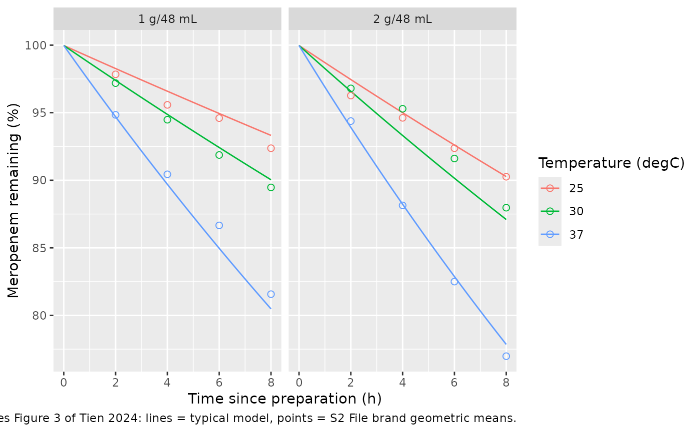
fig3_check <- observed_fig3 |>
  left_join(stab_sim |> select(time = time_bottle, temp, strength, pct_pred),
            by = c("time", "temp", "strength")) |>
  mutate(diff_pct_points = pct_pred - pct_obs)
knitr::kable(fig3_check, digits = 2)| strength | temp | time | n_brands | pct_obs | pct_pred | diff_pct_points |
|---|---|---|---|---|---|---|
| 1 g/48 mL | 25 | 2 | 7 | 97.84 | 98.27 | 0.43 |
| 1 g/48 mL | 25 | 4 | 7 | 95.58 | 96.59 | 1.01 |
| 1 g/48 mL | 25 | 6 | 6 | 94.60 | 94.94 | 0.34 |
| 1 g/48 mL | 25 | 8 | 7 | 92.37 | 93.32 | 0.95 |
| 1 g/48 mL | 30 | 2 | 6 | 97.19 | 97.39 | 0.20 |
| 1 g/48 mL | 30 | 4 | 6 | 94.48 | 94.88 | 0.40 |
| 1 g/48 mL | 30 | 6 | 7 | 91.87 | 92.42 | 0.55 |
| 1 g/48 mL | 30 | 8 | 7 | 89.47 | 90.04 | 0.57 |
| 1 g/48 mL | 37 | 2 | 7 | 94.84 | 94.70 | -0.14 |
| 1 g/48 mL | 37 | 4 | 7 | 90.44 | 89.70 | -0.74 |
| 1 g/48 mL | 37 | 6 | 7 | 86.66 | 84.96 | -1.70 |
| 1 g/48 mL | 37 | 8 | 7 | 81.57 | 80.48 | -1.09 |
| 2 g/48 mL | 25 | 2 | 7 | 96.27 | 97.46 | 1.19 |
| 2 g/48 mL | 25 | 4 | 7 | 94.62 | 95.00 | 0.38 |
| 2 g/48 mL | 25 | 6 | 7 | 92.37 | 92.61 | 0.24 |
| 2 g/48 mL | 25 | 8 | 7 | 90.26 | 90.27 | 0.01 |
| 2 g/48 mL | 30 | 2 | 7 | 96.80 | 96.59 | -0.21 |
| 2 g/48 mL | 30 | 4 | 7 | 95.29 | 93.31 | -1.98 |
| 2 g/48 mL | 30 | 6 | 7 | 91.61 | 90.15 | -1.46 |
| 2 g/48 mL | 30 | 8 | 6 | 87.97 | 87.10 | -0.87 |
| 2 g/48 mL | 37 | 2 | 7 | 94.38 | 93.91 | -0.47 |
| 2 g/48 mL | 37 | 4 | 7 | 88.14 | 88.22 | 0.08 |
| 2 g/48 mL | 37 | 6 | 7 | 82.50 | 82.87 | 0.37 |
| 2 g/48 mL | 37 | 8 | 7 | 76.98 | 77.85 | 0.87 |
stopifnot(
  !anyNA(fig3_check$pct_pred),
  abs(median(fig3_check$diff_pct_points)) < 1,
  max(abs(fig3_check$diff_pct_points)) < 3
)
The fixed effects reproduce the brand-averaged data to within about one percentage point; both sides are deterministic (typical model against tabulated means), so a tight bound is appropriate.
Deterministic profiles (replicates Figure 4A)
Total daily dose 3 g as 375 mg every 3 h, 750 mg every 6 h or 1000 mg every 8 h, each bottle infused over its whole renewal interval, after the 500 mg loading dose.
ci_regimens <- regimens |> filter(grepl("^CI", regimen))
det_grid <- tidyr::crossing(ci_regimens, conditions)
det_events <- bind_rows(lapply(seq_len(nrow(det_grid)), function(i) {
  g <- det_grid[i, ]
  build_events(1, g$interval, g$tinf, g$dose, g$degrade, g$temp, g$strength) |>
    mutate(id = i)
}))
det_sim <- solve_typical(det_events) |>
  left_join(det_grid |> mutate(id = row_number()), by = "id")
#> ℹ omega/sigma items treated as zero: 'etainfusion_log_intercept', 'etakdeg', 'etalcl', 'etalvc', 'etalvp', 'etaiov_cl_1'

det_plot <- det_sim |> filter(condition != "No degradation")
ref_plot <- det_sim |> filter(condition == "No degradation", regimen == "CI 8 h") |>
  select(time, Cc)
ggplot(det_plot, aes(time, Cc)) +
  geom_line(data = ref_plot, colour = "red") +
  geom_line(aes(colour = regimen)) +
  facet_grid(strength ~ temp) +
  scale_colour_grey(start = 0.75, end = 0) +
  labs(x = "Time (h)", y = "Meropenem concentration (mg/L)",
       colour = "Bottle renewal",
       caption = "Replicates Figure 4A of Tien 2024 (red: no degradation).")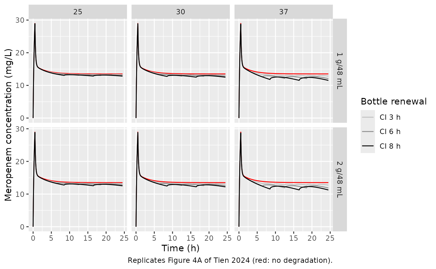
# Peak after the loading dose and the no-degradation steady state.
ref_ss <- det_sim |> filter(condition == "No degradation", regimen == "CI 8 h")
peak_ld <- max(ref_ss$Cc[ref_ss$time <= 1])
css_24 <- ref_ss$Cc[ref_ss$time == 24]
c(peak_after_LD = peak_ld, Css_no_degradation = css_24,
  expected_Css = 125 / 9.25)
#>      peak_after_LD Css_no_degradation       expected_Css
#>           28.98595           13.51456           13.51351
stopifnot(abs(css_24 / (125 / 9.25) - 1) < 0.02, peak_ld > 26, peak_ld < 32)
The no-degradation curve settles at the infusion rate over clearance (125 mg/h / 9.25 L/h = 13.5 mg/L) and peaks near 29 mg/L at the end of the loading dose, as in Figure 4A.
Trough ratio Cmin / Cno-deg (replicates Figure 4B)
Figure 4B shows the concentration at the end of a steady-state bottle (the minimum of the saw-tooth) as a percentage of the no-degradation concentration. The paper’s points are per-brand conditional modes; the maintainers digitised the centre of each brand cluster.
fig4b_digitised <- tibble::tribble(
  ~strength,   ~temp, ~regimen, ~ratio_paper,
  "1 g/48 mL", 25, "CI 3 h", 98.0,
  "1 g/48 mL", 30, "CI 3 h", 97.5,
  "1 g/48 mL", 37, "CI 3 h", 95.2,
  "1 g/48 mL", 25, "CI 6 h", 96.2,
  "1 g/48 mL", 30, "CI 6 h", 94.4,
  "1 g/48 mL", 37, "CI 6 h", 89.8,
  "1 g/48 mL", 25, "CI 8 h", 94.8,
  "1 g/48 mL", 30, "CI 8 h", 92.2,
  "1 g/48 mL", 37, "CI 8 h", 86.0,
  "2 g/48 mL", 25, "CI 3 h", 97.3,
  "2 g/48 mL", 30, "CI 3 h", 96.9,
  "2 g/48 mL", 37, "CI 3 h", 94.3,
  "2 g/48 mL", 25, "CI 6 h", 94.6,
  "2 g/48 mL", 30, "CI 6 h", 93.4,
  "2 g/48 mL", 37, "CI 6 h", 87.6,
  "2 g/48 mL", 25, "CI 8 h", 92.8,
  "2 g/48 mL", 30, "CI 8 h", 91.0,
  "2 g/48 mL", 37, "CI 8 h", 83.0
)

ref_cc <- det_sim |> filter(condition == "No degradation") |>
  select(regimen, time, Cc_ref = Cc)
ratio_sim <- det_sim |>
  filter(condition != "No degradation", time >= 16.5, time <= 24.5) |>
  left_join(ref_cc, by = c("regimen", "time")) |>
  group_by(regimen, temp, strength) |>
  summarise(ratio_model = 100 * min(Cc / Cc_ref), .groups = "drop")

fig4b <- fig4b_digitised |>
  left_join(ratio_sim, by = c("regimen", "temp", "strength")) |>
  mutate(diff = ratio_model - ratio_paper)
knitr::kable(fig4b, digits = 1)| strength | temp | regimen | ratio_paper | ratio_model | diff |
|---|---|---|---|---|---|
| 1 g/48 mL | 25 | CI 3 h | 98.0 | 98.4 | 0.4 |
| 1 g/48 mL | 30 | CI 3 h | 97.5 | 97.5 | 0.0 |
| 1 g/48 mL | 37 | CI 3 h | 95.2 | 95.0 | -0.2 |
| 1 g/48 mL | 25 | CI 6 h | 96.2 | 96.5 | 0.3 |
| 1 g/48 mL | 30 | CI 6 h | 94.4 | 94.7 | 0.3 |
| 1 g/48 mL | 37 | CI 6 h | 89.8 | 89.3 | -0.5 |
| 1 g/48 mL | 25 | CI 8 h | 94.8 | 95.0 | 0.2 |
| 1 g/48 mL | 30 | CI 8 h | 92.2 | 92.6 | 0.4 |
| 1 g/48 mL | 37 | CI 8 h | 86.0 | 85.3 | -0.7 |
| 2 g/48 mL | 25 | CI 3 h | 97.3 | 97.6 | 0.3 |
| 2 g/48 mL | 30 | CI 3 h | 96.9 | 96.8 | -0.1 |
| 2 g/48 mL | 37 | CI 3 h | 94.3 | 94.3 | 0.0 |
| 2 g/48 mL | 25 | CI 6 h | 94.6 | 94.8 | 0.2 |
| 2 g/48 mL | 30 | CI 6 h | 93.4 | 93.0 | -0.4 |
| 2 g/48 mL | 37 | CI 6 h | 87.6 | 87.8 | 0.2 |
| 2 g/48 mL | 25 | CI 8 h | 92.8 | 92.8 | 0.0 |
| 2 g/48 mL | 30 | CI 8 h | 91.0 | 90.4 | -0.6 |
| 2 g/48 mL | 37 | CI 8 h | 83.0 | 83.3 | 0.3 |
The 5-18% reduction stated in the Results is reproduced, rising with the renewal interval and the temperature.
Probability of target attainment (replicates Figures 5 and 6)
Monte Carlo simulation of the first treatment day with IIV on CL, Vc
and Vp and IOV on CL. Target: total concentration above the MIC for at
least 98% of the 0.1 h grid over 0-24 h (S4 File
Cp_GT_MIC). The paper used 1000 patients per regimen and
condition; this vignette uses 200, and every arm of a figure reuses the
same 200 patients through a common seed.
n_mc <- 200

simulate_arm <- function(regimen_row, condition_row, crcl, seed = 2024) {
  ev <- build_events(n_mc, regimen_row$interval, regimen_row$tinf,
                     regimen_row$dose, condition_row$degrade,
                     condition_row$temp, condition_row$strength,
                     crcl = crcl, obs_times = seq(0, 24, by = 0.1))
  rxode2::rxSetSeed(seed)
  rxSolve(mod, ev, returnType = "data.frame", useLinCmt = FALSE) |>
    select(id, time, Cc) |>
    mutate(regimen = regimen_row$regimen, condition = condition_row$condition,
           CRCL = crcl)
}

pta_table <- function(sim, mic) {
  sim |>
    group_by(regimen, condition, CRCL, id) |>
    summarise(ft = 100 * mean(Cc > mic), .groups = "drop") |>
    group_by(regimen, condition, CRCL) |>
    summarise(PTA = 100 * mean(ft >= 98), .groups = "drop") |>
    mutate(MIC = mic)
}
fig5_cond <- conditions |>
  filter(condition %in% c("No degradation", "25 degC - 1 g/48 mL",
                          "37 degC - 2 g/48 mL"))
fig5_sim <- bind_rows(lapply(seq_len(nrow(regimens)), function(i) {
  bind_rows(lapply(seq_len(nrow(fig5_cond)), function(j) {
    simulate_arm(regimens[i, ], fig5_cond[j, ], crcl = 80.8)
  }))
}))
fig5_pta <- bind_rows(lapply(c(2, 4, 8, 16), function(m) pta_table(fig5_sim, m)))

ggplot(fig5_pta, aes(factor(regimen, levels = regimens$regimen), PTA,
                     colour = condition, group = condition)) +
  geom_line() + geom_point() +
  geom_hline(yintercept = 90, linetype = "dashed") +
  facet_wrap(~MIC, nrow = 1, labeller = label_both) +
  labs(x = NULL, y = "PTA day 1, 98% fT>MIC (%)", colour = NULL,
       caption = "Replicates Figure 5 of Tien 2024 (CRCL 80.8 mL/min, WT 70 kg, albumin 2.8 g/dL).") +
  theme(axis.text.x = element_text(angle = 45, hjust = 1), legend.position = "bottom")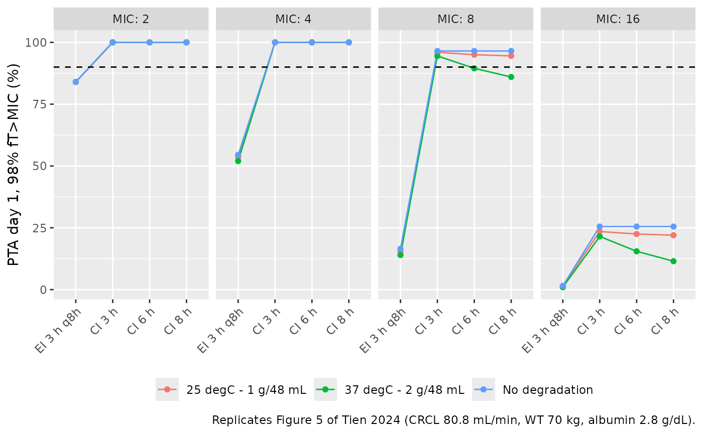
fig5_digitised <- tibble::tribble(
  ~regimen,     ~condition,             ~MIC, ~PTA_paper,
  "EI 3 h q8h", "No degradation",          2,   86,
  "EI 3 h q8h", "No degradation",          4,   59,
  "EI 3 h q8h", "37 degC - 2 g/48 mL",     4,   53,
  "EI 3 h q8h", "No degradation",          8,   17,
  "CI 3 h",     "No degradation",          8,   96,
  "CI 8 h",     "No degradation",          8,   96,
  "CI 8 h",     "25 degC - 1 g/48 mL",     8,   93,
  "CI 8 h",     "37 degC - 2 g/48 mL",     8,   86,
  "CI 3 h",     "No degradation",         16,   25,
  "CI 8 h",     "No degradation",         16,   25,
  "CI 8 h",     "37 degC - 2 g/48 mL",    16,   11
)
fig5_cmp <- fig5_digitised |>
  left_join(fig5_pta |> select(regimen, condition, MIC, PTA_model = PTA),
            by = c("regimen", "condition", "MIC")) |>
  mutate(diff = PTA_model - PTA_paper)
knitr::kable(fig5_cmp, digits = 1)| regimen | condition | MIC | PTA_paper | PTA_model | diff |
|---|---|---|---|---|---|
| EI 3 h q8h | No degradation | 2 | 86 | 84.0 | -2.0 |
| EI 3 h q8h | No degradation | 4 | 59 | 54.5 | -4.5 |
| EI 3 h q8h | 37 degC - 2 g/48 mL | 4 | 53 | 52.0 | -1.0 |
| EI 3 h q8h | No degradation | 8 | 17 | 16.5 | -0.5 |
| CI 3 h | No degradation | 8 | 96 | 96.5 | 0.5 |
| CI 8 h | No degradation | 8 | 96 | 96.5 | 0.5 |
| CI 8 h | 25 degC - 1 g/48 mL | 8 | 93 | 94.5 | 1.5 |
| CI 8 h | 37 degC - 2 g/48 mL | 8 | 86 | 86.0 | 0.0 |
| CI 3 h | No degradation | 16 | 25 | 25.5 | 0.5 |
| CI 8 h | No degradation | 16 | 25 | 25.5 | 0.5 |
| CI 8 h | 37 degC - 2 g/48 mL | 16 | 11 | 11.5 | 0.5 |
stopifnot(
  !anyNA(fig5_cmp$PTA_model),
  abs(median(fig5_cmp$diff)) < 8,
  quantile(abs(fig5_cmp$diff), 0.9) < 20
)
fig6_cond <- conditions |> filter(condition %in% c("No degradation", "37 degC - 2 g/48 mL"))
ci8 <- regimens |> filter(regimen == "CI 8 h")
fig6_sim <- bind_rows(lapply(c(10, 30, 60, 90, 120, 150), function(cr) {
  bind_rows(lapply(seq_len(nrow(fig6_cond)), function(j) {
    simulate_arm(ci8, fig6_cond[j, ], crcl = cr)
  }))
}))
fig6_pta <- bind_rows(lapply(c(4, 8, 16), function(m) pta_table(fig6_sim, m)))

ggplot(fig6_pta, aes(CRCL, PTA, colour = condition)) +
  geom_line() + geom_point() +
  geom_hline(yintercept = 90, linetype = "dashed") +
  facet_wrap(~MIC, labeller = label_both) +
  labs(x = "CRCL (mL/min)", y = "PTA day 1, 98% fT>MIC (%)", colour = NULL,
       caption = "Replicates Figure 6 of Tien 2024 (CI, 1 g every 8 h).") +
  theme(legend.position = "bottom")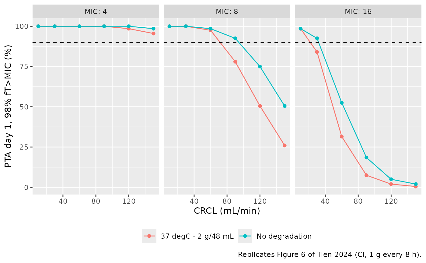
fig6_digitised <- tibble::tribble(
  ~CRCL, ~condition,             ~MIC, ~PTA_paper,
     90, "No degradation",          8,   93,
    120, "No degradation",          8,   74,
    150, "No degradation",          8,   50,
     90, "37 degC - 2 g/48 mL",     8,   80,
    120, "37 degC - 2 g/48 mL",     8,   48,
    150, "37 degC - 2 g/48 mL",     8,   26,
     30, "No degradation",         16,   90,
     60, "No degradation",         16,   45,
     60, "37 degC - 2 g/48 mL",    16,   33
)
fig6_cmp <- fig6_digitised |>
  left_join(fig6_pta |> select(CRCL, condition, MIC, PTA_model = PTA),
            by = c("CRCL", "condition", "MIC")) |>
  mutate(diff = PTA_model - PTA_paper)
knitr::kable(fig6_cmp, digits = 1)| CRCL | condition | MIC | PTA_paper | PTA_model | diff |
|---|---|---|---|---|---|
| 90 | No degradation | 8 | 93 | 92.5 | -0.5 |
| 120 | No degradation | 8 | 74 | 75.0 | 1.0 |
| 150 | No degradation | 8 | 50 | 50.5 | 0.5 |
| 90 | 37 degC - 2 g/48 mL | 8 | 80 | 78.0 | -2.0 |
| 120 | 37 degC - 2 g/48 mL | 8 | 48 | 50.5 | 2.5 |
| 150 | 37 degC - 2 g/48 mL | 8 | 26 | 26.0 | 0.0 |
| 30 | No degradation | 16 | 90 | 92.5 | 2.5 |
| 60 | No degradation | 16 | 45 | 52.5 | 7.5 |
| 60 | 37 degC - 2 g/48 mL | 16 | 33 | 31.5 | -1.5 |
stopifnot(
  !anyNA(fig6_cmp$PTA_model),
  abs(median(fig6_cmp$diff)) < 8,
  quantile(abs(fig6_cmp$diff), 0.9) < 20
)
With 200 patients the Monte Carlo standard error of a PTA near 50% is about 3.5 percentage points, and the digitised values carry a further 1-2 points, so the checks bound the centre and a robust quantile of the differences rather than every point.
NCA of the typical-patient day 1 (PKNCA)
The paper reports no NCA. PKNCA is used here to quantify how much
exposure the bottle loses. For a linear model, the day-1 AUC equals the
drug that reached the patient minus the drug still in the body at 24 h,
divided by clearance; the delivered amount has a closed form, because a
bottle hung at s with dose D and length
T has delivered D * (1 - exp(-k t)) / (k T) by
t = min(T, 24 - s) hours.
nca_conc <- det_sim |>
  filter(!is.na(Cc), time <= 24) |>
  mutate(treatment = paste(regimen, condition, sep = " | ")) |>
  select(id, time, Cc, treatment, regimen, condition)
conc_obj <- PKNCAconc(nca_conc, Cc ~ time | treatment + id)
intervals <- data.frame(start = 0, end = 24, auclast = TRUE, cmax = TRUE)
nca_res <- pk.nca(PKNCAdata(conc_obj, intervals = intervals))
#> No dose information provided, calculations requiring dose will return NA.
nca_wide <- as.data.frame(nca_res) |>
  select(treatment, PPTESTCD, PPORRES) |>
  tidyr::pivot_wider(names_from = PPTESTCD, values_from = PPORRES) |>
  tidyr::separate(treatment, c("regimen", "condition"), sep = " \\| ")

kdeg_typ <- function(temp, strength) {
  0.0086083 + 0.0044789 * (temp == 30) + 0.0185050 * (temp == 37) +
    0.0041512 * (strength == "2 g/48 mL")
}

# Drug delivered by 24 h from every bottle hung before then.
delivered_by_24 <- function(interval, tinf, dose, k) {
  doses <- dose_table(interval, tinf, dose, t_end = 24)
  tau <- pmin(doses$tinf, 24 - doses$time)
  sum(doses$amt * (1 - exp(-k * tau)) / (k * doses$tinf))
}

body_24 <- det_sim |>
  filter(time == 24) |>
  transmute(regimen, condition, body_amount = central + peripheral1)

auc_check <- nca_wide |>
  left_join(nca_wide |> filter(condition == "No degradation") |>
              select(regimen, auc_ref = auclast), by = "regimen") |>
  left_join(conditions, by = "condition") |>
  left_join(regimens, by = "regimen") |>
  left_join(body_24, by = c("regimen", "condition")) |>
  filter(degrade) |>
  rowwise() |>
  mutate(
    delivered = delivered_by_24(interval, tinf, dose, kdeg_typ(temp, strength)),
    auc_mass_balance = (delivered - body_amount) / 9.25
  ) |>
  ungroup() |>
  mutate(
    auc_ratio = auclast / auc_ref,
    pct_diff = 100 * (auclast / auc_mass_balance - 1)
  )
auc_check |>
  select(regimen, condition, cmax, auclast, auc_mass_balance, pct_diff, auc_ratio) |>
  dplyr::rename(
    "Bottle renewal" = regimen, "Condition" = condition,
    "Cmax (mg/L)" = cmax, "AUC0-24 PKNCA (mg*h/L)" = auclast,
    "AUC0-24 mass balance (mg*h/L)" = auc_mass_balance,
    "Difference (%)" = pct_diff,
    "AUC0-24 ratio vs no degradation" = auc_ratio
  ) |>
knitr::kable(digits = 3)| Bottle renewal | Condition | Cmax (mg/L) | AUC0-24 PKNCA (mg*h/L) | AUC0-24 mass balance (mg*h/L) | Difference (%) | AUC0-24 ratio vs no degradation |
|---|---|---|---|---|---|---|
| CI 3 h | 25 degC - 1 g/48 mL | 28.909 | 332.896 | 332.930 | -0.010 | 0.989 |
| CI 3 h | 25 degC - 2 g/48 mL | 28.871 | 331.161 | 331.196 | -0.011 | 0.984 |
| CI 3 h | 30 degC - 1 g/48 mL | 28.868 | 331.024 | 331.060 | -0.011 | 0.984 |
| CI 3 h | 30 degC - 2 g/48 mL | 28.831 | 329.303 | 329.340 | -0.011 | 0.978 |
| CI 3 h | 37 degC - 1 g/48 mL | 28.743 | 325.264 | 325.304 | -0.012 | 0.966 |
| CI 3 h | 37 degC - 2 g/48 mL | 28.706 | 323.589 | 323.630 | -0.013 | 0.962 |
| CI 6 h | 25 degC - 1 g/48 mL | 28.909 | 329.588 | 329.621 | -0.010 | 0.979 |
| CI 6 h | 25 degC - 2 g/48 mL | 28.871 | 326.316 | 326.351 | -0.011 | 0.970 |
| CI 6 h | 30 degC - 1 g/48 mL | 28.868 | 326.060 | 326.094 | -0.011 | 0.969 |
| CI 6 h | 30 degC - 2 g/48 mL | 28.831 | 322.843 | 322.879 | -0.011 | 0.959 |
| CI 6 h | 37 degC - 1 g/48 mL | 28.743 | 315.390 | 315.429 | -0.012 | 0.937 |
| CI 6 h | 37 degC - 2 g/48 mL | 28.706 | 312.339 | 312.378 | -0.013 | 0.928 |
| CI 8 h | 25 degC - 1 g/48 mL | 28.909 | 327.478 | 327.512 | -0.010 | 0.973 |
| CI 8 h | 25 degC - 2 g/48 mL | 28.871 | 323.247 | 323.281 | -0.011 | 0.961 |
| CI 8 h | 30 degC - 1 g/48 mL | 28.868 | 322.917 | 322.951 | -0.011 | 0.960 |
| CI 8 h | 30 degC - 2 g/48 mL | 28.831 | 318.779 | 318.814 | -0.011 | 0.947 |
| CI 8 h | 37 degC - 1 g/48 mL | 28.743 | 309.273 | 309.311 | -0.012 | 0.919 |
| CI 8 h | 37 degC - 2 g/48 mL | 28.706 | 305.414 | 305.453 | -0.013 | 0.908 |
The PKNCA AUC agrees with the mass balance to within the trapezoidal error of the 0.1 h grid, so the bottle delivers exactly the drug the stability model says survives. Over the first day the loss ranges from about 1% (3 h bottles at 25 degC) to about 9% (8 h bottles at 37 degC, 2 g/48 mL).
Assumptions and deviations
- PK layer from the S4 File, not from Ehmann 2019 itself. Ehmann 2019 (doi:10.1016/j.ijantimicag.2019.06.016) is not open access and was not available; every PK value comes from Tien’s RxODE recoding, which matches the summary of the same model in Yang et al. 2022 (Front Pharmacol 13:838205, Table 2), apart from Yang printing the albumin centring as 2.79 g/dL where Tien uses 2.8. Re-verify against Ehmann 2019 when it is obtained.
-
Above the CRCL hinge. Tien’s code sets CL to
CLCR_INF * 60 / 1000(9.24 L/h) above 154 mL/min, a discontinuous drop from 15.9 L/h just below it that none of the paper’s simulations reach (all use CRCL <= 150). Yang 2022 prints “CL = CL-INF” for this branch. The model holds CL at its value at the hinge, the continuous reading of the published relationship. -
Residual error on Cc is not reported in Tien 2024
or its supplements, so
propSdisfixed(0); the paper’s PTA simulations used individual predictions without residual error, as here. -
IOV on CL enters as one occasion
(
etaiov_cl_1), as Tien simulated only the first treatment day; for multi-day simulation the occasion structure of Ehmann 2019 would be needed. - Bottle random effects. The stability model’s random intercept and slope are per bottle series. Tien’s simulations used the typical kdeg (or per-brand conditional modes in Figure 4B); in a stochastic simulation of this model each patient also draws a bottle kdeg, which changes kdeg by about 0.0015 1/h (1 SD) and has no visible effect on PTA. The intercept describes the measured log(C/C0) at preparation and does not scale the delivered dose.
-
Albumin units. The source model takes albumin in
g/dL; the canonical
ALBcolumn is g/L and is divided by 10 in the model. - Brand. Tested and not retained (Model 4, p = 0.14), so it is not a covariate.
-
S3 File parameter table. The knitted
df_stability_paramtable in S3 File shows the 37 degC and 2 g/48 mL coefficients on every row, because itsifelse()compares the labelled factor levels (‘25 degC’, ‘1g/48mL’) with bare numbers. Figure 4 clearly differs by temperature, so the simulations did not use those printed rows; the model uses thesummary(fit3)coefficients, which agree with Table 2. - Figures 4B, 5 and 6 were digitised by the maintainers from the published images (about 1-2 percentage points of reading error).