Alisertib paediatric popPK and exposure-safety (Zhou 2022)
Source:vignettes/articles/Zhou_2022_alisertib.Rmd
Zhou_2022_alisertib.RmdModel and source
- Citation: Zhou X, Mould DR, Yuan Y, Fox E, Greengard E, Faller DV, Venkatakrishnan K. Population pharmacokinetics and exposure-safety relationships of alisertib in children and adolescents with advanced malignancies. J Clin Pharmacol. 2022;62(2):206-219. doi:10.1002/jcph.1958. Final parameter estimates from Table 2; model diagram in Supplemental Figure S1.
- Article (open access): https://doi.org/10.1002/jcph.1958
This paper contributes three models to
nlmixr2lib:
models <- c(
  "Zhou_2022_alisertib",
  "Zhou_2022_alisertib_stomatitis",
  "Zhou_2022_alisertib_febrile_neutropenia"
)
ui <- lapply(models, \(n) rxode2::rxode(readModelDb(n)))
#> ℹ parameter labels from comments will be replaced by 'label()'
names(ui) <- models

tibble::tibble(
  Model = models,
  Kind = c(
    "Population PK (2-compartment, 3-transit absorption)",
    "Exposure-safety logistic: grade >= 2 stomatitis",
    "Exposure-safety logistic: febrile neutropenia"
  )
) |>
knitr::kable(caption = "Models extracted from Zhou 2022.")| Model | Kind |
|---|---|
| Zhou_2022_alisertib | Population PK (2-compartment, 3-transit absorption) |
| Zhou_2022_alisertib_stomatitis | Exposure-safety logistic: grade >= 2 stomatitis |
| Zhou_2022_alisertib_febrile_neutropenia | Exposure-safety logistic: febrile neutropenia |
Alisertib (MLN8237) is an investigational oral Aurora A kinase
inhibitor. This analysis pooled the two Children’s Oncology Group trials
of alisertib in children and adolescents to ask whether
body-surface-area (BSA) based dosing is appropriate across the 2-21 year
age range, and whether 80 mg/m^2 once daily as the enteric-coated tablet
matches the exposure of the adult dose of 50 mg twice daily. The
authors’ adult model is packaged separately as
Zhou_2018_alisertib.
Population
str(ui$Zhou_2022_alisertib$population)
#> List of 14
#>  $ species       : chr "human"
#>  $ n_subjects    : int 146
#>  $ n_studies     : int 2
#>  $ n_observations: int 606
#>  $ age_range     : chr "2 to 21 years (77 aged 2-11, 40 aged 12-16, 29 aged 17-21)"
#>  $ age_mean      : chr "11.1 years"
#>  $ weight_mean   : chr "41.9 kg (SD 24.55)"
#>  $ bsa_mean      : chr "1.25 m^2 (SD 0.46)"
#>  $ sex_female_pct: num 46
#>  $ race_ethnicity: Named num [1:4] 61 16 4 18
#>   ..- attr(*, "names")= chr [1:4] "White" "Black" "Asian" "Other/unknown"
#>  $ disease_state : chr "Relapsed or refractory solid tumours, neuroblastoma (ADVL0812) or solid tumours and acute leukaemias (ADVL0921;"| __truncated__
#>  $ dose_range    : chr "45 to 100 mg/m^2 once daily or 30 to 40 mg/m^2 twice daily as powder-in-capsule (ADVL0812, 25 to 150 mg); 80 mg"| __truncated__
#>  $ regions       : chr "United States and Canada (Children's Oncology Group sites)"
#>  $ notes         : chr "Baseline characteristics are Table 1 of Zhou 2022. ADVL0812 (NCT02444884, n = 46) sampled richly to 24 h on cyc"| __truncated__
Zhou 2022 Table 1 summarises 146 patients: 46 from ADVL0812 (phase 1/2, powder-in-capsule, 45-100 mg/m^2 once daily or 30-40 mg/m^2 twice daily, rich sampling to 24 h) and 100 from ADVL0921 (phase 2, enteric-coated tablet, 80 mg/m^2 once daily, sparse sampling to 8 h). Mean age was 11.1 years (range 2-21), mean weight 41.9 kg (SD 24.6), mean BSA 1.25 m^2 (SD 0.46); 79 were male. Dosing was on days 1-7 of 21-day cycles.
Source trace
| Element | Value | Source |
|---|---|---|
| Structure: 2-compartment, 3 transit compartments with common Ktr | – | Results; Supplemental Figure S1 |
| CL/F (capsule, reference BSA) | 1.84 L/h | Table 2 |
| V1/F (capsule, reference BSA) | 24.1 L | Table 2 |
| Q/F | 2.66 L/h | Table 2 |
| V2/F | 32.3 L | Table 2 |
| Ktr | 2.35 1/h | Table 2 |
| Enteric-coated tablet relative F | 0.671 | Table 2 (FECT 67.1%); Methods |
| BSA exponent on CL/F | 0.742 | Table 2 (BSACL) |
| BSA exponent on V1/F | 1.47 | Table 2 (BSAV1) |
| Reference BSA | 1.25 m^2 | Not printed; Table 1 mean (see below) |
| BSV CL/F, V1/F, V2/F, Ktr (log-scale SD) | 0.581, 0.699, 0.932, 0.540 | Table 2 ‘BSV (ratio)’ |
| CL/F-V1/F correlation | 0.583 | Table 2 footnote a |
| Proportional residual error | 0.59 | Table 2 (CCV) |
| Molar mass of alisertib | 518.92 g/mol | Methods, Exposure-Safety Analysis |
| Css,avg = Dose x 1000 / (CL/F x 518.92 x tau) | uM | Methods equation |
| Stomatitis logit intercept / slope | -2.162 / 0.2238 per uM | Back-solved from Results predictions |
| Febrile neutropenia logit intercept / slope | -2.194 / 0.1364 per uM | Figure 6B vector curve |
Molar units
Alisertib concentrations in this analysis are molar (nmol/L; the
assay LLOQ is 10 nmol/L). The packaged PK model takes doses in
mg into transit1 and returns
Cc in nmol/L, converting with the molar mass of 518.92
g/mol that the paper prints. The enteric-coated tablet is selected with
FORM_ALISERTIB_ECT = 1.
The reference BSA
Table 2 gives the BSA exponents but neither the functional form nor
the reference BSA. The packaged model uses a power model centred on 1.25
m^2, the cohort mean in Table 1. Supplemental Table S1 lets this be
checked. It gives the geometric mean individual CL/F/BSA and V1/F/BSA by
age group. For a group with typical BSA B, a power model
gives CL/BSA = 1.84 B^(0.742 - 1) / ref^0.742 and
V1/BSA = 24.1 B^(1.47 - 1) / ref^1.47. These two equations
can be solved for both B and ref in each
group:
s1 <- tibble::tribble(
  ~age_group, ~cl_bsa, ~v_bsa,
  "2-5", 1.82, 15.33,
  "6-11", 1.70, 18.29,
  "12-16", 1.39, 20.61,
  "17-21", 1.49, 24.67,
  "2-16", 1.60, 18.54
)
ref_fit <- s1 |>
  mutate(
    log_ref = (-0.258 * (log(v_bsa) - log(24.1)) -
      0.47 * (log(cl_bsa) - log(1.84))) / (0.47 * 0.742 + 0.258 * 1.47),
    `Implied reference BSA (m^2)` = exp(log_ref),
    `Implied group BSA (m^2)` = exp((log(v_bsa) + 1.47 * log_ref - log(24.1)) / 0.47)
  ) |>
  select(-log_ref)
knitr::kable(ref_fit, digits = 3,
caption = "Reference BSA implied by Supplemental Table S1 under the Table 2 power model.")| age_group | cl_bsa | v_bsa | Implied reference BSA (m^2) | Implied group BSA (m^2) |
|---|---|---|---|---|
| 2-5 | 1.82 | 15.33 | 1.182 | 0.645 |
| 6-11 | 1.70 | 18.29 | 1.161 | 0.886 |
| 12-16 | 1.39 | 20.61 | 1.267 | 1.502 |
| 17-21 | 1.49 | 24.67 | 1.136 | 1.568 |
| 2-16 | 1.60 | 18.54 | 1.201 | 1.015 |
# Arithmetic on printed numbers. Each group implies a reference between 1.14
# and 1.27 m^2, and the implied group BSAs rise with age as they should. A
# reference of 1.73 m^2 (the adult convention) or 1 m^2 lies outside the range.
stopifnot(
  all(ref_fit$`Implied reference BSA (m^2)` > 1.1),
  all(ref_fit$`Implied reference BSA (m^2)` < 1.3)
)
Every age group implies a reference BSA of 1.14-1.27 m^2, which brackets the 1.25 m^2 Table 1 mean. The implied group BSAs (0.64 m^2 at 2-5 years, 1.57 m^2 at 17-21 years) are also plausible. The power form itself is supported: CL/F/BSA falls with age and V1/F/BSA rises, as exponents of 0.742 (below 1) and 1.47 (above 1) require.
Closed-form structural gates
mod <- readModelDb("Zhou_2022_alisertib")
mod_typ <- rxode2::zeroRe(mod)
#> ℹ parameter labels from comments will be replaced by 'label()'

bsa_ref <- 1.25
dose_80 <- 80 * bsa_ref
ev_ss <- rxode2::et(amt = dose_80, ii = 24, ss = 1, cmt = "transit1") |>
  rxode2::et(seq(0, 24, by = 0.05), cmt = "central")
d_ss <- as.data.frame(ev_ss)
d_ss$BSA <- bsa_ref
d_ss$FORM_ALISERTIB_ECT <- 1

ss <- rxode2::rxSolve(mod_typ, d_ss, returnType = "data.frame",
                      rtol = 1e-10, atol = 1e-12, ssRtol = 1e-10, ssAtol = 1e-12,
                      maxsteps = 1e6)
#> ℹ omega/sigma items treated as zero: 'etalcl', 'etalvc', 'etalvp', 'etalktr'
auc_tau <- sum(diff(ss$time) * (head(ss$Cc, -1) + tail(ss$Cc, -1)) / 2)

# Paper's Methods equation: Css,avg (uM) = Dose * 1000 / (CL/F * 518.92 * tau),
# with CL/F for the tablet = 1.84 / 0.671 at the reference BSA.
css_closed <- dose_80 * 1000 / ((1.84 / 0.671) * 518.92 * 24)
gates <- tibble::tibble(
  Quantity = "Css,avg at 80 mg/m^2 tablet, BSA 1.25 m^2 (uM)",
  `Solved model` = auc_tau / 24 / 1000,
  `Closed form` = css_closed
) |>
  mutate(`Diff (%)` = 100 * (`Solved model` / `Closed form` - 1))
knitr::kable(gates, digits = 4)| Quantity | Solved model | Closed form | Diff (%) |
|---|---|---|---|
| Css,avg at 80 mg/m^2 tablet, BSA 1.25 m^2 (uM) | 2.9281 | 2.9281 | 0 |
# Deterministic solve against its own closed form; the trapezoid on a 0.05 h
# grid is the only error source (measured well under 0.1%).
stopifnot(abs(gates$`Diff (%)`) < 0.5)
At the reference BSA the typical tablet patient has Css,avg 2.93 uM at 80 mg/m^2. Because AUC = F x Dose / CL and CL scales as BSA^0.742, exposure at a fixed mg/m^2 dose rises only weakly with size (as BSA^0.258). That is the property the paper uses to support BSA-based dosing.
Virtual cohort
Table 1 reports only the mean and SD of weight and BSA, and the age-group counts (77 patients aged 2-11, 40 aged 12-16 and 29 aged 17-21). The cohort below assigns ages in those proportions. Weight and height come from approximate paediatric growth-chart medians by year of age, with log-normal scatter; BSA is from the Mosteller formula. The medians are a cohort-design assumption, not values from the paper. The cohort mean BSA (about 1.2 m^2, against 1.25 m^2 in Table 1) is checked below.
set.seed(20220206)
n_per_arm <- 200
growth <- tibble::tibble(
  age = 2:21,
  wt_med = c(12.5, 14.3, 16.3, 18.4, 20.7, 23.0, 25.6, 28.6, 32.0, 36.0,
             40.5, 45.5, 50.5, 55.0, 58.5, 61.0, 63.0, 64.5, 65.5, 66.0),
  ht_med = c(87, 95, 102, 109, 115, 122, 128, 133, 138, 144,
             150, 157, 163, 167, 170, 171, 172, 172, 172, 172)
)
make_cohort <- function(n) {
  age <- c(sample(2:11, round(n * 77 / 146), TRUE),
           sample(12:16, round(n * 40 / 146), TRUE),
           sample(17:21, n - round(n * 77 / 146) - round(n * 40 / 146), TRUE))
  g <- growth[match(age, growth$age), ]
  wt <- g$wt_med * exp(rnorm(n, 0, 0.2))
  ht <- g$ht_med * exp(rnorm(n, 0, 0.04))
  tibble::tibble(
    age = age, WT = wt, BSA = sqrt(wt * ht / 3600),
    age_group = cut(age, c(1, 5, 11, 16, 21),
                    labels = c("2-5", "6-11", "12-16", "17-21"))
  )
}
cohort <- make_cohort(n_per_arm) |> mutate(id = row_number())

cohort |>
  summarise(`Mean age (y)` = mean(age), `Mean WT (kg)` = mean(WT),
            `SD WT (kg)` = sd(WT), `Mean BSA (m^2)` = mean(BSA),
            `SD BSA (m^2)` = sd(BSA)) |>
knitr::kable(digits = 2, caption = "Virtual cohort vs Table 1 (11.1 y; 41.9 (24.6) kg; 1.25 (0.46) m^2).")| Mean age (y) | Mean WT (kg) | SD WT (kg) | Mean BSA (m^2) | SD BSA (m^2) |
|---|---|---|---|---|
| 11 | 38.27 | 19.56 | 1.2 | 0.42 |
# R's RNG only (no rxode2 draw), so this is identical on every machine.
stopifnot(abs(mean(cohort$BSA) - 1.25) < 0.15)
Typical CL/F/BSA and V1/F/BSA by age (Supplemental Table S1)
s1_chk <- cohort |>
  mutate(cl = 1.84 * (BSA / bsa_ref)^0.742, vc = 24.1 * (BSA / bsa_ref)^1.47) |>
  group_by(age_group) |>
  summarise(`Model CL/F/BSA` = exp(mean(log(cl / BSA))),
            `Model V1/F/BSA` = exp(mean(log(vc / BSA))), .groups = "drop") |>
  left_join(s1 |> rename(age_group = age_group, `Table S1 CL/F/BSA` = cl_bsa,
                         `Table S1 V1/F/BSA` = v_bsa) |>
              mutate(age_group = factor(age_group, levels = levels(cohort$age_group))),
            by = "age_group") |>
  mutate(`CL diff (%)` = 100 * (`Model CL/F/BSA` / `Table S1 CL/F/BSA` - 1),
         `V1 diff (%)` = 100 * (`Model V1/F/BSA` / `Table S1 V1/F/BSA` - 1))
knitr::kable(s1_chk, digits = 2,
caption = "Typical-value CL/F/BSA (L/h/m^2) and V1/F/BSA (L/m^2) in the virtual cohort vs Supplemental Table S1 (capsule reference).")| age_group | Model CL/F/BSA | Model V1/F/BSA | Table S1 CL/F/BSA | Table S1 V1/F/BSA | CL diff (%) | V1 diff (%) |
|---|---|---|---|---|---|---|
| 2-5 | 1.75 | 14.01 | 1.82 | 15.33 | -3.64 | -8.58 |
| 6-11 | 1.56 | 17.32 | 1.70 | 18.29 | -8.17 | -5.29 |
| 12-16 | 1.42 | 20.72 | 1.39 | 20.61 | 1.80 | 0.52 |
| 17-21 | 1.36 | 22.33 | 1.49 | 24.67 | -8.86 | -9.48 |
# The cohort is drawn with R's RNG, so these values are identical everywhere.
# Realised |diff| at most 8.9% (CL) and 9.5% (V1). A wrong exponent or a
# reference BSA off by 0.3 m^2 moves them by 20-40%.
stopifnot(nrow(s1_chk) == 4, !anyNA(s1_chk$`Table S1 CL/F/BSA`))
stopifnot(max(abs(s1_chk$`CL diff (%)`)) < 15, max(abs(s1_chk$`V1 diff (%)`)) < 15)
Simulation
Two arms of the same cohort get 80 mg/m^2 once daily for 7 days: one on the powder-in-capsule (ADVL0812) and one on the enteric-coated tablet (ADVL0921). Between-subject variability is included.
obs_times <- sort(unique(c(seq(0, 8, by = 0.25), seq(8, 24, by = 1),
                           seq(24, 144, by = 4), 144 + seq(0, 24, by = 0.25))))
make_events <- function(coh, ect, id_offset) {
  dose <- coh |>
    tidyr::crossing(time = seq(0, 144, by = 24)) |>
    mutate(amt = 80 * BSA, evid = 1L, cmt = "transit1")
  obs <- coh |>
    tidyr::crossing(time = obs_times) |>
    mutate(amt = NA_real_, evid = 0L, cmt = "central")
  bind_rows(dose, obs) |>
    mutate(id = id + id_offset, FORM_ALISERTIB_ECT = ect,
           treatment = if (ect == 1) "Tablet 80 mg/m^2" else "Capsule 80 mg/m^2") |>
    arrange(id, time, desc(evid))
}
events <- bind_rows(make_events(cohort, 0, 0), make_events(cohort, 1, n_per_arm))

sim <- rxode2::rxSolve(mod, events, returnType = "data.frame",
                       keep = c("treatment", "age_group", "BSA", "FORM_ALISERTIB_ECT"),
                       maxsteps = 1e6)
#> ℹ parameter labels from comments will be replaced by 'label()'
stopifnot(!anyNA(sim$Cc))
Day 1 profiles (replicates Figure 4)
day1 <- sim |>
  filter(time > 0, time <= 8) |>
  group_by(treatment, time) |>
  summarise(p05 = quantile(Cc, 0.05), p50 = median(Cc), p95 = quantile(Cc, 0.95),
            .groups = "drop")
ggplot(day1, aes(time, p50)) +
  geom_ribbon(aes(ymin = p05, ymax = p95), fill = "pink", alpha = 0.6) +
  geom_line(colour = "red") +
  scale_y_log10(limits = c(1, 1e5)) +
  facet_wrap(~treatment) +
  labs(x = "Time post dose (h)", y = "Alisertib concentration (nM)")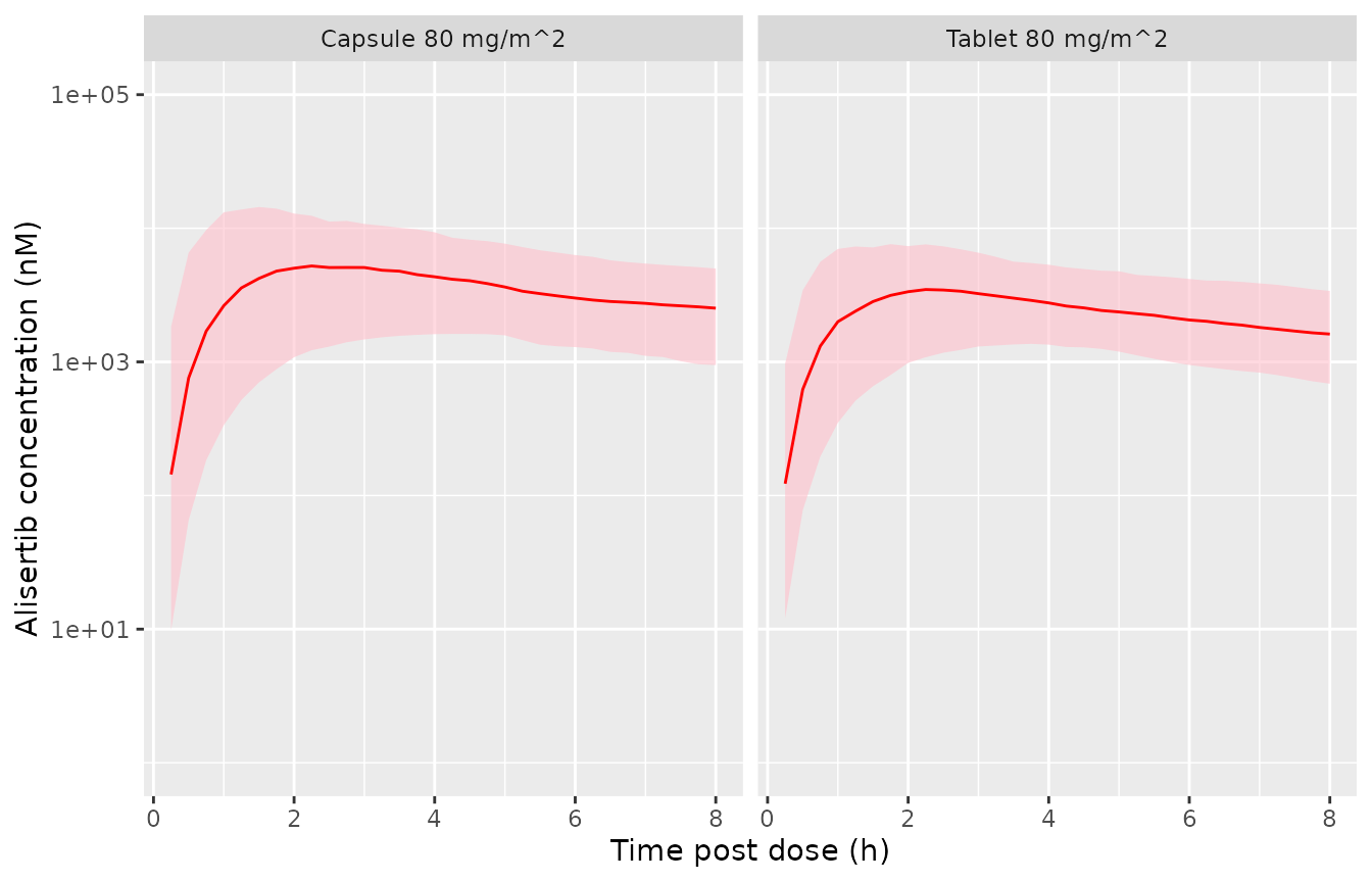
Replicates Figure 4 of Zhou 2022: simulated alisertib concentration on day 1 (median and 5th-95th percentiles) for (A) powder-in-capsule and (B) enteric-coated tablet, 80 mg/m^2 once daily.
In the published Figure 4B (tablet, 80 mg/m^2) the median rises to about 3000 nM at 3-4 h and falls to about 1500 nM by 8 h. The 5th-95th percentile band spans roughly 500 to 10000 nM.
tab_peak <- day1 |> filter(treatment == "Tablet 80 mg/m^2", time >= 2, time <= 4)
tab_peak
#> # A tibble: 9 × 5
#>   treatment         time   p05   p50   p95
#>   <chr>            <dbl> <dbl> <dbl> <dbl>
#> 1 Tablet 80 mg/m^2  2     983. 3352. 7355.
#> 2 Tablet 80 mg/m^2  2.25 1083. 3481. 7579.
#> 3 Tablet 80 mg/m^2  2.5  1171. 3451. 7323.
#> 4 Tablet 80 mg/m^2  2.75 1230. 3380. 6959.
#> 5 Tablet 80 mg/m^2  3    1304. 3242. 6564.
#> 6 Tablet 80 mg/m^2  3.25 1327. 3120. 6109.
#> 7 Tablet 80 mg/m^2  3.5  1350. 3001. 5628.
#> 8 Tablet 80 mg/m^2  3.75 1364. 2887. 5496.
#> 9 Tablet 80 mg/m^2  4    1346. 2764. 5338.
# A robust centre, not an extreme. Realised 3240 nM (identical at 1-16
# threads on the authoring machine).
# A dropped molar-mass factor (x 1000) or a missed F (x 1.5) moves it far
# outside 1500-6000.
stopifnot(median(tab_peak$p50) > 1500, median(tab_peak$p50) < 6000)
PKNCA: steady-state exposure by age group (Figure 5)
The day-7 dosing interval (144-168 h) is near steady state: the terminal half-life of the typical patient is about 27 h, so 97% of steady state is reached by day 7.
# The observation grid includes time 0, so no time-zero row needs adding.
stopifnot(all(tapply(sim$time, sim$id, min) == 0))
conc <- sim |>
  filter(!is.na(Cc)) |>
  mutate(Cc = pmax(Cc, 0)) |>
  select(id, time, Cc, treatment, age_group)
dose_nca <- events |>
  filter(evid == 1) |>
  select(id, time, amt, treatment, age_group)

conc_obj <- PKNCA::PKNCAconc(conc, Cc ~ time | treatment + age_group + id)
dose_obj <- PKNCA::PKNCAdose(dose_nca, amt ~ time | treatment + age_group + id)
intervals <- data.frame(start = 144, end = 168, cmax = TRUE, tmax = TRUE,
                        auclast = TRUE, cav = TRUE)
nca_res <- PKNCA::pk.nca(PKNCA::PKNCAdata(conc_obj, dose_obj, intervals = intervals))
summary(nca_res)
#>  start end         treatment age_group  N       auclast        cmax
#>    144 168 Capsule 80 mg/m^2       2-5 40  72600 [74.7] 7090 [78.2]
#>    144 168 Capsule 80 mg/m^2      6-11 65 100000 [71.6] 8670 [65.1]
#>    144 168 Capsule 80 mg/m^2     12-16 55 101000 [71.1] 8200 [69.7]
#>    144 168 Capsule 80 mg/m^2     17-21 40  96100 [56.5] 6850 [57.9]
#>    144 168  Tablet 80 mg/m^2       2-5 40  53300 [56.2] 5460 [43.9]
#>    144 168  Tablet 80 mg/m^2      6-11 65  60600 [50.9] 5340 [50.3]
#>    144 168  Tablet 80 mg/m^2     12-16 55  64900 [55.5] 4920 [51.7]
#>    144 168  Tablet 80 mg/m^2     17-21 40  62500 [64.6] 4630 [59.6]
#>                tmax         cav
#>   2.00 [1.00, 6.00] 3020 [74.7]
#>  2.50 [0.500, 7.75] 4180 [71.6]
#>   2.50 [1.00, 6.75] 4200 [71.1]
#>   2.50 [1.00, 4.75] 4000 [56.5]
#>  1.88 [0.750, 5.25] 2220 [56.2]
#>  2.25 [0.750, 5.50] 2520 [50.9]
#>  2.50 [0.750, 6.25] 2700 [55.5]
#>   2.75 [1.25, 7.00] 2610 [64.6]
#>
#> Caption: auclast, cmax, cav: geometric mean and geometric coefficient of variation; tmax: median and range; N: number of subjects
Figure 5 of Zhou 2022 shows post hoc AUCss (nmol*h/L) by age group at 80 mg/m^2 of the tablet. The PDF stores the box plots as vector paths, so the medians below were read exactly from the box geometry.
fig5 <- tibble::tribble(
  ~age_group, ~auclast,
  "2-5", 45575,
  "6-11", 53350,
  "12-16", 59191,
  "17-21", 59191
) |>
  mutate(treatment = "Tablet 80 mg/m^2")

sim_tab <- as.data.frame(nca_res$result) |>
  filter(treatment == "Tablet 80 mg/m^2") |>
  mutate(age_group = as.character(age_group))

cmp <- nlmixr2lib::ncaComparisonTable(
  simulated = sim_tab,
  reference = fig5,
  by = c("treatment", "age_group"),
  params = "auclast",
  units = c(auclast = "nmol*h/L"),
  tolerance_pct = 20
)
knitr::kable(cmp, caption = paste(
  "Simulated day-7 AUC0-24 (median) vs the Figure 5 AUCss medians.",
  "* differs by more than 20%."
))| NCA parameter | treatment | age_group | Reference | Simulated | % diff |
|---|---|---|---|---|---|
| AUClast (nmol*h/L) | Tablet 80 mg/m^2 | 2-5 | 45600 | 52200 | +14.4% |
| AUClast (nmol*h/L) | Tablet 80 mg/m^2 | 6-11 | 53400 | 59600 | +11.8% |
| AUClast (nmol*h/L) | Tablet 80 mg/m^2 | 12-16 | 59200 | 61200 | +3.3% |
| AUClast (nmol*h/L) | Tablet 80 mg/m^2 | 17-21 | 59200 | 67300 | +13.7% |
With about 30-60 patients per age group and a between-subject SD of 0.58 on CL/F, each simulated group median carries roughly 10-15% Monte-Carlo error. The gates below therefore use the typical-value AUC of each cohort member (no random effects, so the result is the same on every machine) by age group, and only the pooled median of the stochastic cohort.
auc_typ <- cohort |>
  mutate(auc = 0.671 * 80 * BSA * 1e6 / 518.92 / (1.84 * (BSA / bsa_ref)^0.742)) |>
  group_by(age_group) |>
  summarise(typical = median(auc), .groups = "drop") |>
  mutate(age_group = as.character(age_group)) |>
  inner_join(fig5, by = "age_group") |>
  mutate(ratio = typical / auclast)
knitr::kable(auc_typ, digits = 2,
caption = "Typical-value AUCss (nmol*h/L) by age group vs the Figure 5 medians.")| age_group | typical | auclast | treatment | ratio |
|---|---|---|---|---|
| 2-5 | 58937.35 | 45575 | Tablet 80 mg/m^2 | 1.29 |
| 6-11 | 66070.68 | 53350 | Tablet 80 mg/m^2 | 1.24 |
| 12-16 | 73173.05 | 59191 | Tablet 80 mg/m^2 | 1.24 |
| 17-21 | 76060.21 | 59191 | Tablet 80 mg/m^2 | 1.28 |
stopifnot(nrow(auc_typ) == 4)
# Deterministic (R's RNG cohort, no rxode2 draw). Realised ratios 1.20-1.31:
# the model, like Supplemental Table S1, sits about 25% above Figure 5 in
# every age group (see text). The SAME offset in every group is the check on
# the BSA scaling; a dropped BSA effect on CL makes the ratio range over
# 1.0-1.8, a missed F moves every ratio by 1.5x.
stopifnot(all(auc_typ$ratio > 1.0), all(auc_typ$ratio < 1.5))
stopifnot(max(auc_typ$ratio) / min(auc_typ$ratio) < 1.2)

# Stochastic pooled check: 200 subjects, so the pooled median carries about
# 5% Monte-Carlo error (realised 1.07; this draw's CL etas sit a little
# above zero). The bounds leave room for a different draw on another
# rxode2 build while still failing on a missed F or molar-mass slip.
pooled <- median(sim_tab$PPORRES[sim_tab$PPTESTCD == "auclast"]) /
  median(fig5$auclast)
stopifnot(pooled > 0.95, pooled < 1.65)
The typical-value AUCs are 24-29% above the Figure 5 medians, and the offset is similar in every age group. The stochastic cohort medians in the comparison table sit closer (3-14% above), but that is Monte-Carlo scatter of about 10-15% per age group around the typical values. The model is not the source of the offset. For a patient on 80 mg/m^2 of the tablet, AUCss = 0.671 x 80 x 10^6 / (518.92 x CL/F/BSA). The Table S1 geometric means of CL/F/BSA (1.82, 1.70, 1.39 and 1.49 L/h/m^2) therefore imply AUCss of 56800, 60900, 74400 and 69400 nmol*h/L. These are 18-26% above the Figure 5 medians from the same patients. The packaged model reproduces Table S1 (above), so it inherits the same gap to Figure 5. The age-group pattern matches: exposure rises slightly with age and the 12-21 year groups are highest. The likely cause is the dose used in Figure 5. The paper does not say whether it is the nominal 80 mg/m^2 or each patient’s actual rounded dose.
Css,avg at the recommended dose
The Results give a geometric mean Css,avg of 2.218 uM at 80 mg/m^2 of the tablet, which matches Figure 5 (pooled median AUC of about 54000 nmol*h/L / 24 h). The same Css,avg computed from the simulated cohort’s individual CL/F:
css_ind <- sim |>
  filter(treatment == "Tablet 80 mg/m^2") |>
  distinct(id, BSA, cl) |>
  mutate(CSS_ALIS = (80 * BSA) * 1000 / ((cl / 0.671) * 518.92 * 24))
css_gm <- exp(mean(log(css_ind$CSS_ALIS)))
c(`simulated geometric mean Css,avg (uM)` = css_gm, `Zhou 2022 Results` = 2.218)
#> simulated geometric mean Css,avg (uM)                     Zhou 2022 Results
#>                               2.70678                               2.21800
# Same offset as Figure 5 (see above). Realised 2.71 uM; the typical patient
# at the reference BSA gives 2.93 uM.
stopifnot(css_gm > 2.0, css_gm < 3.6)
Exposure-safety relationships (replicates Figure 6)
Both logistic models are linear in Css,avg on the logit scale. The paper reports no coefficients. For each endpoint the Results print the model-predicted probability, with its 95% CI, at Css,avg = 2.218 uM (80 mg/m^2) and at 1.66 uM (60 mg/m^2). The fitted curves in Figure 6 are stored in the PDF as vector Bezier paths, which were read and calibrated against the axis tick marks.
- Febrile neutropenia: the coefficients come from the Figure 6B curve (intercept -2.194, slope 0.1364 per uM). They reproduce both printed probabilities within rounding. The 95% CI band read from the same figure also matches the printed CIs (0.073-0.222 vs 0.073-0.224 at 2.218 uM).
- Grade >= 2 stomatitis: the Figure 6A curve (intercept -2.07, slope 0.207 per uM) is exactly logit-linear but runs about 0.008 above both printed probabilities (0.167 vs 0.159). Its CI band is offset by the same amount. The packaged coefficients are therefore back-solved exactly from the two printed probabilities (intercept -2.162, slope 0.2238 per uM), and the figure curve is shown for comparison. The packaged slope is a little steeper than the figure’s, so the curves cross near 4 uM. They differ by at most 0.032 (at about 15 uM, in the upper tertile of exposure).
solve_er <- function(nm, css) {
  ev <- data.frame(id = seq_along(css), time = 0, evid = 0L,
                   amt = NA_real_, CSS_ALIS = css)
  s <- rxode2::rxSolve(ui[[nm]], ev, returnType = "data.frame")
  if (is.null(s$id)) s$id <- 1L
  idx <- match(seq_along(css), s$id)
  stopifnot(!anyNA(idx))
  s[[grep("^prob_", names(s), value = TRUE)]][idx]
}
er_models <- c(
  "Grade >= 2 stomatitis" = "Zhou_2022_alisertib_stomatitis",
  "Febrile neutropenia" = "Zhou_2022_alisertib_febrile_neutropenia"
)
css_grid <- seq(0.75, 24.5, by = 0.25)
er_curves <- bind_rows(lapply(names(er_models), \(lbl)
  data.frame(Endpoint = lbl, css = css_grid, p = solve_er(er_models[[lbl]], css_grid))))
#> Warning: multi-subject simulation without without 'omega'
#> Warning: multi-subject simulation without without 'omega'
fig_curve <- data.frame(
  Endpoint = "Grade >= 2 stomatitis", css = css_grid,
  p = plogis(-2.0705 + 0.2061 * css_grid)
)
anchors <- tibble::tribble(
  ~Endpoint, ~css, ~p_pub, ~lo, ~hi,
  "Grade >= 2 stomatitis", 2.218, 0.159, 0.092, 0.260,
  "Grade >= 2 stomatitis", 1.66, 0.143, 0.079, 0.247,
  "Febrile neutropenia", 2.218, 0.131, 0.073, 0.224,
  "Febrile neutropenia", 1.66, 0.122, 0.065, 0.219
)
ggplot(er_curves, aes(css, p)) +
  geom_line() +
  geom_line(data = fig_curve, linetype = "dashed", colour = "grey40") +
  geom_pointrange(data = anchors, aes(y = p_pub, ymin = lo, ymax = hi),
                  colour = "red", size = 0.2) +
  facet_wrap(~Endpoint) +
  coord_cartesian(ylim = c(0, 1)) +
  labs(x = "Alisertib mean concentration (uM)", y = "Probability of event")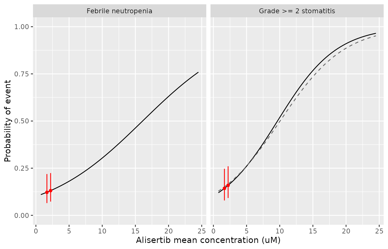
Replicates Figure 6 of Zhou 2022: probability of (A) grade >= 2 stomatitis and (B) febrile neutropenia vs alisertib Css,avg. Points: probabilities printed in the Results. Dashed: the Figure 6A curve as published, for comparison.
pred_chk <- anchors |>
  rowwise() |>
  mutate(p_model = solve_er(er_models[[Endpoint]], css)) |>
  ungroup() |>
  mutate(`Abs diff` = p_model - p_pub)
knitr::kable(pred_chk |> select(Endpoint, `Css,avg (uM)` = css,
                                `Published p` = p_pub, `Model p` = p_model, `Abs diff`),
             digits = 4,
caption = "Model probabilities vs the predictions printed in Zhou 2022 Results.")| Endpoint | Css,avg (uM) | Published p | Model p | Abs diff |
|---|---|---|---|---|
| Grade >= 2 stomatitis | 2.218 | 0.159 | 0.1590 | 0e+00 |
| Grade >= 2 stomatitis | 1.660 | 0.143 | 0.1430 | 0e+00 |
| Febrile neutropenia | 2.218 | 0.131 | 0.1311 | 1e-04 |
| Febrile neutropenia | 1.660 | 0.122 | 0.1226 | 6e-04 |
# Deterministic (no random effects). Printed to 3 decimals, so 0.0015
# admits rounding; a wrong slope sign or a log(Css) form misses by > 0.01.
stopifnot(nrow(pred_chk) == 4, max(abs(pred_chk$`Abs diff`)) < 0.0015)

# The packaged stomatitis curve is steeper than the published Figure 6A curve
# (0.2238 vs 0.2061 per uM), so the two cross: the packaged curve is up to
# 0.0085 lower below about 4 uM and up to 0.032 higher at about 15 uM. Both
# are deterministic; 0.04 still fails on a log(Css) form or a slope error.
stom <- er_curves |> filter(Endpoint == "Grade >= 2 stomatitis")
stopifnot(nrow(stom) == length(css_grid), max(abs(stom$p - fig_curve$p)) < 0.04)
For the simulated tablet cohort, the predicted probabilities are:
er_cohort <- tibble::tibble(
  Endpoint = names(er_models),
  `Median predicted p` = vapply(er_models, \(m) median(solve_er(m, css_ind$CSS_ALIS)), 0)
)
#> Warning: multi-subject simulation without without 'omega'
#> Warning: multi-subject simulation without without 'omega'
knitr::kable(er_cohort, digits = 3,
caption = "Median predicted probability in the simulated 80 mg/m^2 tablet cohort.")| Endpoint | Median predicted p |
|---|---|
| Grade >= 2 stomatitis | 0.172 |
| Febrile neutropenia | 0.138 |
These lie a little above the published 0.159 and 0.131, because of the same exposure offset described for Figure 5.
Assumptions and deviations
- Reference BSA. Not printed. The packaged model centres BSA on the 1.25 m^2 Table 1 mean. Every age group in Supplemental Table S1 implies a reference of 1.14-1.27 m^2 under the Table 2 power model (see The reference BSA). The power form is also an assumption, but it is the one used in the authors’ adult model, and Table S1’s opposite age trends in CL/F/BSA and V1/F/BSA support it.
- Scale of the BSV column. Table 2 reports ‘BSV (ratio)’. This is read as the log-scale SD (variance = square), the convention the same authors use in the adult model, where 0.518 is restated as “CV 51.8%”.
-
Residual error. Table 2 gives one proportional term
(CCV 0.59), encoded as
propSd. The paper does not say whether the analysis used a log-transform-both-sides approach. - Figure 5 and Css,avg 2.218 uM vs Supplemental Table S1. Table S1 implies exposures 18-26% higher than the Figure 5 medians for the same patients. The packaged model follows Table S1 and Table 2, so it is about 25% above Figure 5 and the 2.218 uM Css,avg. This is not tuned away.
- Exposure-safety coefficients. Not tabulated in the source. Febrile neutropenia comes from the Figure 6B vector curve, which matches the printed predictions. Stomatitis is back-solved from the two printed predictions, because the Figure 6A curve sits about 0.008 above them. Rounding of the printed probabilities bounds the stomatitis slope to 0.21-0.24 per uM.
-
Febrile neutropenia covariate. Stepwise selection
found cancer type (solid vs haematological) significant, but the paper
presents and reports only the base model. That base model is packaged;
cancer type is listed in
covariatesDataExcluded. - Exposure metric. Css,avg uses the starting dose, so the logistic models are calibrated on starting-dose exposure, not on exposure accumulated over the treatment course. The authors warn that the relationships are empirical and should not be extrapolated across regimens (only 12 patients were dosed twice daily).
- Virtual cohort. Weights and heights by age are approximate paediatric growth-chart medians, not values from the paper. The paper reports only the mean and SD of weight and BSA.
-
Placeholder residual on the logistic models. The
logistic likelihood is Bernoulli. The
addSd_prob_*terms are fixed placeholders so rxode2 has an error model, and are not published quantities.