Ceftobiprole (Cojutti 2023)
Source:vignettes/articles/Cojutti_2023_ceftobiprole.Rmd
Cojutti_2023_ceftobiprole.RmdModel and source
- Citation: Cojutti PG, Giuliano S, Pascale R, Angelini J, Tascini C, Viale P, Pea F. Population Pharmacokinetic and Pharmacodynamic Analysis for Maximizing the Effectiveness of Ceftobiprole in the Treatment of Severe Methicillin-Resistant Staphylococcal Infections. Microorganisms. 2023;11(12):2964. doi:10.3390/microorganisms11122964
- Description: Three-compartment IV population PK model for ceftobiprole in adults with severe Gram-positive infections (real-life multicentre therapeutic drug monitoring cohort, Italy). Clearance rises exponentially with CKD-EPI estimated glomerular filtration rate; central volume V1 is larger in males. Supports probability-of-target-attainment analysis against free-trough or free-steady-state fCtrough/MIC and fCss/MIC targets.
- Article: https://doi.org/10.3390/microorganisms11122964
Cojutti and colleagues fitted a three-compartment intravenous population PK model to routine therapeutic drug monitoring (TDM) data from two Italian tertiary hospitals, then used it in Monte Carlo simulations to ask which ceftobiprole regimens attain aggressive beta-lactam PK/PD targets. Two covariates were retained: CKD-EPI estimated glomerular filtration rate on clearance, and sex on the central volume.
Population
A total of 132 adults contributing 503 ceftobiprole plasma concentrations were included (Table 1). The median (IQR) age was 71.0 (61.8-79.0) years, body weight 73.5 (65.0-89.0) kg, and CKD-EPI eGFR 83.7 (50.5-101.7) mL/min/1.73 m^2; 86 were male and 46 female (34.8% female). Ceftobiprole was given for severe Gram-positive infection, most often hospital-acquired pneumonia (28.8%), endocarditis (20.5%), bloodstream infection (16.6%), and community-acquired pneumonia (15.2%). Starting regimens were adjusted by renal function and given as 3 h extended infusions: 500 mg q8h at eGFR >= 50, 500 mg q12h at eGFR 30-50, and 250 mg q12h at eGFR < 30 mL/min/1.73 m^2, with subsequent TDM-guided adjustment. The median (IQR) daily dose was 1500 (1000-1500) mg.
The same information is available programmatically via the model’s
population metadata
(readModelDb("Cojutti_2023_ceftobiprole")()$population).
Source trace
Every ini() entry carries an in-file comment naming its
source location in
inst/modeldb/specificDrugs/Cojutti_2023_ceftobiprole.R.
They are collected here for review. All structural, covariate, IIV, and
residual values come from the “Covariate Model Estimate (%
RSE)” column of Table 2, i.e. the paper’s final model.
| Equation / parameter | Value | Source location |
|---|---|---|
lcl (CL intercept at CRCL = 0) |
1.7 L/h | Table 2, covariate model, CL (11.9% RSE) |
lvc (V1, female reference) |
14.77 L | Table 2, covariate model, V1 (19.7% RSE) |
lq (Q2) |
6.11 L/h | Table 2, covariate model, Q2 (13.6% RSE) |
lvp (V2) |
46.16 L | Table 2, covariate model, V2 (34.8% RSE) |
lq2 (Q3) |
42.41 L/h | Table 2, covariate model, Q3 (61.6% RSE) |
lvp2 (V3) |
4.76 L | Table 2, covariate model, V3 (13.9% RSE) |
e_crcl_cl (eGFR on CL) |
0.011 per mL/min/1.73 m^2 | Table 2, covariate effect (12.6% RSE) |
e_sex_vc (male sex on V1) |
0.39 | Table 2, covariate effect (54.8% RSE) |
etalcl variance |
0.202676 (47.4 %CV) | Table 2, IIV on CL (8.43% RSE) |
etalvc variance |
0.449169 (75.3 %CV) | Table 2, IIV on V1 (19.4% RSE) |
cov(etalcl, etalvc) |
0.181033 (r = 0.6) | Table 2, Correlation CL and V1 (24.8% RSE) |
etalq variance |
0.115558 (35.0 %CV) | Table 2, IIV on Q2 (34.5% RSE) |
etalvp variance |
2.102640 (268.1 %CV) | Table 2, IIV on V2 (19.4% RSE) |
etalq2 variance |
1.876698 (235.2 %CV) | Table 2, IIV on Q3 (45.1% RSE) |
etalvp2 variance |
0.090068 (30.7 %CV) | Table 2, IIV on V3 (30.0% RSE) |
addSd |
1.44 mg/L | Table 2, residual variability a (13.4% RSE) |
propSd |
0.22 | Table 2, residual variability b (5.8% RSE) |
| Three-compartment ODE system | n/a | Methods 2.3 and Results 3.2 (“a three-compartment model”, “zero-order administration and first-order elimination from the central compartment”) |
| Free fraction 0.84 used for PK/PD targets | n/a | Methods 2.4 (“assuming a 16% protein binding”) |
Covariate functional form: reconciling the text with the numbers
Results section 3.2 states the covariates were added “as a power function of ceftobiprole CL and V1, respectively”. The reported coefficient of 0.011 cannot be a power exponent. Under any power parameterization the eGFR effect would be numerically negligible, which contradicts both the abstract (“Estimated glomerular filtration rate significantly affected drug clearance”) and the paper’s own reported median individual CL of 4.04 L/h (Results 3.2).
The discriminator is V2: it carries no covariate, so its typical value (46.16 L) and its reported median individual value (46.6 L) should agree – and they do, to 1.0%. That establishes “median individual value ~= typical value” as a reliable check in this paper. Scoring each candidate form for CL against the reported 4.04 L/h at the cohort median eGFR of 83.7:
egfr_med <- 83.7   # Table 1 median eGFR
cl_pop   <- 1.7    # Table 2 covariate model CL
beta     <- 0.011  # Table 2 eGFR on CL
target   <- 4.04   # Results 3.2 median individual CL

# Formula labels avoid the asterisk: knitr::kable() emits markdown, where a
# paired "*" is rendered as emphasis and silently disappears from the table.
forms <- tibble::tribble(
  ~form,                                       ~cl,
  "exponential  1.7 x exp(0.011 x eGFR)",      cl_pop * exp(beta * egfr_med),
  "power (/70)  1.7 x (eGFR/70)^0.011",        cl_pop * (egfr_med / 70)^beta,
  "power (/90)  1.7 x (eGFR/90)^0.011",        cl_pop * (egfr_med / 90)^beta,
  "power (raw)  1.7 x eGFR^0.011",             cl_pop * egfr_med^beta,
  "linear add   1.7 + 0.011 x eGFR",           cl_pop + beta * egfr_med,
  "linear mult  1.7 x (1 + 0.011 x eGFR)",     cl_pop * (1 + beta * egfr_med)
) |>
  dplyr::mutate(pct_diff = 100 * (cl - target) / target)

forms |>
  dplyr::rename(
    "Candidate form"            = form,
    "CL at eGFR 83.7 (L/h)"     = cl,
    "% difference vs 4.04 L/h"  = pct_diff
  ) |>
  knitr::kable(digits = c(0, 2, 1),
caption = "Only the exponential form reproduces the paper's own reported median individual CL.")| Candidate form | CL at eGFR 83.7 (L/h) | % difference vs 4.04 L/h |
|---|---|---|
| exponential 1.7 x exp(0.011 x eGFR) | 4.27 | 5.7 |
| power (/70) 1.7 x (eGFR/70)^0.011 | 1.70 | -57.8 |
| power (/90) 1.7 x (eGFR/90)^0.011 | 1.70 | -58.0 |
| power (raw) 1.7 x eGFR^0.011 | 1.78 | -55.8 |
| linear add 1.7 + 0.011 x eGFR | 2.62 | -35.1 |
| linear mult 1.7 x (1 + 0.011 x eGFR) | 3.27 | -19.2 |
The exponential (linear-on-log-scale) form – Monolix’s default for an
untransformed continuous covariate – lands within 5.7%; every
power reading is off by more than 55%. This also explains why the
reported CL falls from 3.43 L/h in the base model to 1.7 L/h in the
covariate model: with an uncentered covariate,
exp(lcl) is the clearance extrapolated to eGFR = 0, not a
typical clearance. The model file therefore encodes
cl = exp(lcl + etalcl) * exp(e_crcl_cl * CRCL).
The same reasoning identifies the sex reference category, which Table 2 does not state:
tibble::tribble(
  ~assignment,          ~v1_female, ~v1_male,
  "female = reference", 14.77,      14.77 * exp(0.39),
  "male = reference",   14.77 * exp(0.39), 14.77
) |>
  # The median subject in an 86-male / 46-female cohort is male, so the
  # predicted median V1 is the male value; the paper reports 19.7 L.
  dplyr::mutate(
    predicted_median_v1 = v1_male,
    pct_diff = 100 * (predicted_median_v1 - 19.7) / 19.7
  ) |>
  dplyr::rename(
    "Assignment"              = assignment,
    "V1 female (L)"           = v1_female,
    "V1 male (L)"             = v1_male,
    "Predicted median V1 (L)" = predicted_median_v1,
    "% difference vs 19.7 L"  = pct_diff
  ) |>
  knitr::kable(digits = c(0, 2, 2, 2, 1),
caption = "Female is the reference category for V1.")| Assignment | V1 female (L) | V1 male (L) | Predicted median V1 (L) | % difference vs 19.7 L |
|---|---|---|---|---|
| female = reference | 14.77 | 21.82 | 21.82 | 10.7 |
| male = reference | 21.82 | 14.77 | 14.77 | -25.0 |
Female-as-reference lands within 10.8% of the reported median;
male-as-reference is 25% low, and the larger male V1 is the
physiologically expected direction. The model file stores sex under the
canonical SEXF (1 = female) and applies the effect as
exp(e_sex_vc * (1 - SEXF)), preserving the published V1 =
14.77 L verbatim.
mod <- readModelDb("Cojutti_2023_ceftobiprole")

ev_chk <- rxode2::et(amt = 500, ii = 8, until = 24, cmt = "central", rate = 500 / 3) |>
  rxode2::et(c(0, 12), cmt = "central")

# Typical values are obtained with `omega = NA` rather than `rxode2::zeroRe()`:
# zeroRe() mutates the model object in place, which would silently strip the
# IIV from every later chunk in this vignette (the cohort, NCA, and PTA
# simulations all reuse `mod`).
typ <- lapply(c(male = 0, female = 1), function(sf) {
  d <- rxode2::rxSolve(mod, ev_chk, params = c(CRCL = 83.7, SEXF = sf),
                       omega = NA, sigma = NA,
                       returnType = "data.frame", addDosing = FALSE)
  tibble::tibble(cl = d$cl[1], vc = d$vc[1], vp = d$vp[1])
}) |> dplyr::bind_rows(.id = "sex")
#> ℹ parameter labels from comments will be replaced by 'label()'

typ |>
  dplyr::rename("Sex" = sex, "CL (L/h)" = cl, "V1 (L)" = vc, "V2 (L)" = vp) |>
  knitr::kable(digits = 2,
caption = "Typical parameters at the cohort median eGFR of 83.7 mL/min/1.73 m^2. Paper Results 3.2 reports median individual CL 4.04 L/h, V1 19.7 L, V2 46.6 L.")| Sex | CL (L/h) | V1 (L) | V2 (L) |
|---|---|---|---|
| male | 4.27 | 21.82 | 46.16 |
| female | 4.27 | 14.77 | 46.16 |
Virtual cohort: reproducing the observed TDM concentrations
Results section 3.2 reports the observed concentration distributions directly: median (min-max) Ctrough 7.4 (0.7-37.2) mg/L, end-of-3 h-infusion 18.4 (4.6-55.3) mg/L, and 1 h post-infusion 14.8 (5.0-55.5) mg/L. These are external data the model file can be checked against.
The cohort below places 200 virtual subjects at deterministic quantiles of the Table 1 eGFR distribution (a piecewise-linear interpolation through the reported Q1 / median / Q3) rather than drawing at random, so the comparison is stable across runs. Sex is assigned to match the 86/46 male/female split, and each subject receives the eGFR-stratified 3 h extended-infusion starting regimen from Methods 2.1.
set.seed(20231212)
n_cohort <- 200

p <- (seq_len(n_cohort) - 0.5) / n_cohort
subj <- tibble::tibble(
  id   = seq_len(n_cohort),
  # Table 1: eGFR median (IQR) 83.7 (50.5-101.7); tails set to a plausible
  # 10-180 mL/min/1.73 m^2 spanning the paper's five simulated renal classes.
  CRCL = stats::approx(x = c(0, 0.25, 0.50, 0.75, 1),
                       y = c(10, 50.5, 83.7, 101.7, 180), xout = p)$y,
  # Table 1: 86 male / 46 female.
  SEXF = as.integer(p > 86 / 132)
) |>
  dplyr::mutate(
    # Methods 2.1 starting regimens, 3 h extended infusion.
    amt_mg = dplyr::if_else(CRCL < 30, 250, 500),
    tau_h  = dplyr::if_else(CRCL >= 50, 8, 12),
    regimen = paste0(amt_mg, " mg q", tau_h, "h 3 h-EI")
  )

# One week of dosing precedes sampling; the last dose is at 168 h and the TDM
# samples are taken over the interval that follows. This mirrors the study,
# where TDM began after at least 2 days of therapy (median treatment duration
# 10 days), rather than assuming exact steady state.
doses <- subj |>
  dplyr::rowwise() |>
  dplyr::reframe(id, CRCL, SEXF, regimen, amt_mg, tau_h,
                 time = seq(0, 168, by = tau_h)) |>
  dplyr::mutate(evid = 1L, amt = amt_mg, cmt = "central", rate = amt_mg / 3)

obs <- subj |>
  dplyr::rowwise() |>
  dplyr::reframe(id, CRCL, SEXF, regimen, amt_mg, tau_h,
                 time = 168 + c(3, 4, tau_h)) |>
  dplyr::mutate(evid = 0L, amt = NA_real_, cmt = "central", rate = NA_real_)

events <- dplyr::bind_rows(doses, obs) |> dplyr::arrange(id, time, dplyr::desc(evid))
stopifnot(!anyDuplicated(unique(events[, c("id", "time", "evid")])))

sim <- rxode2::rxSolve(mod, events = events, keep = c("regimen", "tau_h")) |>
  as.data.frame()

# Guard: between-subject variability must actually be present. If `mod` were
# ever stripped of its random effects (e.g. by an in-place zeroRe() upstream),
# subjects sharing a regimen and eGFR would collapse onto identical profiles
# and every downstream PTA in this vignette would be meaningless.
stopifnot(dplyr::n_distinct(round(sim$cl, 6)) > 0.9 * n_cohort)
tdm <- sim |>
  dplyr::filter(!is.na(Cc)) |>
  dplyr::mutate(
    sample = dplyr::case_when(
      abs(time - 171) < 1e-6                ~ "End of 3 h infusion",
      abs(time - 172) < 1e-6                ~ "1 h post-infusion",
      abs(time - (168 + tau_h)) < 1e-6      ~ "Ctrough"
    )
  ) |>
  dplyr::filter(!is.na(sample)) |>
  dplyr::group_by(sample) |>
  dplyr::summarise(sim_median = median(Cc), sim_min = min(Cc), sim_max = max(Cc),
                   .groups = "drop")

published_obs <- tibble::tribble(
  ~sample,               ~obs_median, ~obs_min, ~obs_max,
  "Ctrough",             7.4,         0.7,      37.2,
  "End of 3 h infusion", 18.4,        4.6,      55.3,
  "1 h post-infusion",   14.8,        5.0,      55.5
)

cmp_obs <- published_obs |>
  dplyr::left_join(tdm, by = "sample") |>
  dplyr::mutate(pct_diff = 100 * (sim_median - obs_median) / obs_median)

cmp_obs |>
  dplyr::select(sample, obs_median, sim_median, pct_diff, obs_min, sim_min, obs_max, sim_max) |>
  dplyr::rename(
    "Sample"                = sample,
    "Observed median"       = obs_median,
    "Simulated median"      = sim_median,
    "% difference"          = pct_diff,
    "Observed min"          = obs_min,
    "Simulated min"         = sim_min,
    "Observed max"          = obs_max,
    "Simulated max"         = sim_max
  ) |>
  knitr::kable(digits = 1,
caption = "Simulated vs. observed ceftobiprole concentrations (mg/L), Cojutti 2023 Results 3.2.")| Sample | Observed median | Simulated median | % difference | Observed min | Simulated min | Observed max | Simulated max |
|---|---|---|---|---|---|---|---|
| Ctrough | 7.4 | 7.0 | -5.4 | 0.7 | 0.3 | 37.2 | 30.0 |
| End of 3 h infusion | 18.4 | 16.0 | -13.1 | 4.6 | 4.4 | 55.3 | 53.7 |
| 1 h post-infusion | 14.8 | 12.6 | -14.6 | 5.0 | 2.1 | 55.5 | 39.2 |
# All three published medians must be reproduced within 20%.
stopifnot(all(abs(cmp_obs$pct_diff) < 20))
All three published medians are reproduced within about 15%, and the simulated min-max ranges track the observed ones. This is an independent corroboration of the exponential eGFR form: under a power reading, clearance would sit near 1.7 L/h and the simulated concentrations would be roughly 2.5-fold too high – an error far larger than the residual discrepancy here. Note that the cohort carries the model’s full between-subject variability (75 %CV on V1), so with 200 subjects the simulated medians themselves carry a Monte Carlo standard error of several percent.
# Companion to Figure 2 of Cojutti 2023 (VPC of concentration vs. time). Here
# the final steady-state dosing interval is shown by starting regimen.
ev_prof <- subj |>
  dplyr::rowwise() |>
  dplyr::reframe(id, CRCL, SEXF, regimen, amt_mg, tau_h,
                 time = c(seq(0, 168, by = tau_h), seq(168, 168 + tau_h, by = 0.25))) |>
  dplyr::mutate(
    evid = dplyr::if_else(time <= 168 & (time %% tau_h == 0), 1L, 0L),
    amt  = dplyr::if_else(evid == 1L, amt_mg, NA_real_),
    rate = dplyr::if_else(evid == 1L, amt_mg / 3, NA_real_),
    cmt  = "central"
  ) |>
  dplyr::distinct(id, time, evid, .keep_all = TRUE) |>
  dplyr::arrange(id, time, dplyr::desc(evid))

sim_prof <- rxode2::rxSolve(mod, events = ev_prof, keep = c("regimen")) |>
  as.data.frame() |>
  dplyr::filter(!is.na(Cc), time >= 168) |>
  dplyr::mutate(tad = time - 168)

sim_prof |>
  dplyr::group_by(regimen, tad) |>
  dplyr::summarise(Q10 = quantile(Cc, 0.10), Q50 = quantile(Cc, 0.50),
                   Q90 = quantile(Cc, 0.90), .groups = "drop") |>
  ggplot(aes(tad, Q50)) +
  geom_ribbon(aes(ymin = Q10, ymax = Q90), alpha = 0.25, fill = "steelblue") +
  geom_line(linewidth = 0.8) +
  facet_wrap(~regimen, scales = "free_x") +
  labs(x = "Time after dose (h)", y = "Ceftobiprole concentration (mg/L)",
       caption = paste("Companion to Figure 2 of Cojutti 2023: 10th / 50th / 90th",
                       "percentiles over the final steady-state dosing interval."))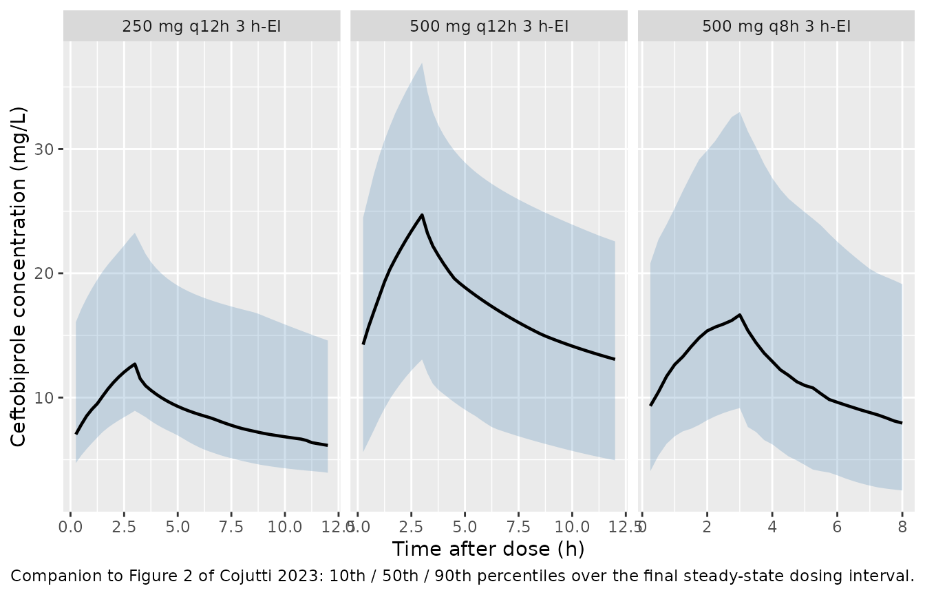
PKNCA validation
For a linear model at steady state, the area under the curve over one
dosing interval is exactly Dose / CL. That identity is an
exact gate on the packaged model, so it is used here in place of a
published NCA table (Cojutti 2023 reports no NCA parameters). Three
uniform dose arms also test dose proportionality.
Subjects are placed at analytic steady state with
ss = 1. This matters: the model’s IIV on V2 is 268 %CV, so
the slowest-distributing subjects have distribution half-lives of
several days and are measurably short of steady state even after a week
of simulated dosing – which would break the identity for reasons that
have nothing to do with the model being wrong.
set.seed(4)
n_arm <- 100
arms <- c(`250 mg q8h` = 250, `500 mg q8h` = 500, `1000 mg q8h` = 1000)
tau  <- 8

# Each arm is solved separately from the SAME seed, so subject k has identical
# random effects in all three arms. That turns dose proportionality into an
# exact per-subject identity rather than a comparison of two independent
# random samples.
#
# Analytic steady state (ss = 1) rather than dosing forward from time zero:
# the IIV on V2 is 268 %CV, so the slowest-distributing subjects are still not
# at steady state after a week of dosing; ss = 1 puts every subject exactly at
# steady state, which is what makes the AUCtau = Dose / CL identity exact.
sim_arm <- function(dose, lbl) {
  base <- tibble::tibble(id = seq_len(n_arm), CRCL = 83.7, SEXF = 0L)
  dose_rows <- base |>
    dplyr::mutate(time = 0, evid = 1L, amt = dose,
                  rate = dose / 2,     # 2 h extended infusion per Methods 2.4
                  ss = 1L, ii = tau, cmt = "central")
  obs_rows <- base |>
    tidyr::crossing(time = seq(0, tau, by = 0.1)) |>
    dplyr::mutate(evid = 0L, amt = NA_real_, rate = NA_real_,
                  ss = 0L, ii = 0, cmt = "central")
  ev <- dplyr::bind_rows(dose_rows, obs_rows) |>
    dplyr::arrange(id, time, dplyr::desc(evid))
  stopifnot(!anyDuplicated(unique(ev[, c("id", "time", "evid")])))
  set.seed(4)
  # Tight tolerances: dose proportionality is asserted per subject to 1e-6,
  # and the ODE at default tolerances lands at 1.6e-6.
  # steady-state searches for long-half-life subjects exceed the default step budget
  rxode2::rxSolve(mod, events = ev, rtol = 1e-10, atol = 1e-12, maxsteps = 1e6) |>
    as.data.frame() |>
    dplyr::mutate(treatment = lbl, amt_mg = dose)
}

sim_nca_raw <- dplyr::bind_rows(
  lapply(names(arms), function(l) sim_arm(unname(arms[[l]]), l))
)

nca_subj <- sim_nca_raw |> dplyr::distinct(treatment, id, amt_mg)

# The shared seed must actually have produced identical individual clearances
# across arms; otherwise the proportionality test below is not exact.
stopifnot(
  sim_nca_raw |>
    dplyr::distinct(treatment, id, cl) |>
    dplyr::group_by(id) |>
    dplyr::summarise(n_cl = dplyr::n_distinct(round(cl, 10)), .groups = "drop") |>
    dplyr::pull(n_cl) |> max() == 1
)
sim_nca <- sim_nca_raw |>
  dplyr::filter(!is.na(Cc)) |>
  dplyr::select(id, time, Cc, treatment)

conc_obj <- PKNCA::PKNCAconc(sim_nca, Cc ~ time | treatment + id)

dose_df <- nca_subj |>
  dplyr::transmute(id, time = 0, amt = amt_mg, treatment)
# duration= is required for an IV infusion so PKNCA does not misplace the input.
dose_obj <- PKNCA::PKNCAdose(dose_df, amt ~ time | treatment + id, duration = 2)

intervals <- data.frame(
  start = 0, end = tau,
  auclast = TRUE, cmax = TRUE, tmax = TRUE, cmin = TRUE
)

nca_res <- PKNCA::pk.nca(PKNCA::PKNCAdata(conc_obj, dose_obj, intervals = intervals))
# PKNCA emits dependency rows; filter on the interval as well as the parameter.
nca_wide <- as.data.frame(nca_res) |>
  dplyr::filter(start == 0, end == tau) |>
  dplyr::select(treatment, id, PPTESTCD, PPORRES) |>
  tidyr::pivot_wider(names_from = PPTESTCD, values_from = PPORRES)

cl_by_id <- sim_nca_raw |>
  dplyr::group_by(treatment, id) |>
  dplyr::summarise(cl = dplyr::first(cl), .groups = "drop")

ident <- nca_wide |>
  dplyr::left_join(cl_by_id, by = c("treatment", "id")) |>
  dplyr::left_join(nca_subj, by = c("treatment", "id")) |>
  dplyr::mutate(auc_theory = amt_mg / cl,
                pct_err = 100 * (auclast - auc_theory) / auc_theory)

ident |>
  dplyr::group_by(treatment) |>
  dplyr::summarise(
    `AUCtau, PKNCA (mg*h/L)`   = median(auclast),
    `AUCtau, Dose/CL (mg*h/L)` = median(auc_theory),
    `Max abs. % error`         = max(abs(pct_err)),
    `Cmax (mg/L)`              = median(cmax),
    `Cmin (mg/L)`              = median(cmin),
    .groups = "drop"
  ) |>
  dplyr::rename("Regimen" = treatment) |>
  knitr::kable(digits = c(0, 1, 1, 4, 2, 2),
caption = "Steady-state NCA vs. the exact linear identity AUCtau = Dose / CL.")| Regimen | AUCtau, PKNCA (mg*h/L) | AUCtau, Dose/CL (mg*h/L) | Max abs. % error | Cmax (mg/L) | Cmin (mg/L) |
|---|---|---|---|---|---|
| 1000 mg q8h | 227.2 | 227.2 | 0.0079 | 42.10 | 18.51 |
| 250 mg q8h | 56.8 | 56.8 | 0.0079 | 10.52 | 4.63 |
| 500 mg q8h | 113.6 | 113.6 | 0.0079 | 21.05 | 9.25 |
# Exact identity: trapezoidal error on a 0.1 h grid must be well under 1%.
stopifnot(max(abs(ident$pct_err)) < 1)

# Dose proportionality, asserted PER SUBJECT (the arms share eta draws), so
# doubling / quadrupling the dose must scale AUCtau exactly for every subject.
prop <- ident |>
  dplyr::select(treatment, id, auclast) |>
  tidyr::pivot_wider(names_from = treatment, values_from = auclast)
r2 <- prop[["500 mg q8h"]]  / prop[["250 mg q8h"]]
r4 <- prop[["1000 mg q8h"]] / prop[["250 mg q8h"]]
stopifnot(max(abs(r2 - 2)) < 1e-6, max(abs(r4 - 4)) < 1e-6)
Replicating the probability of target attainment (Figures 3 and 4)
Methods 2.4 defines the PK/PD targets on the free
concentration (16% protein binding, so fC = 0.84 * Cc)
evaluated at 72 h: quasi-optimal is
fCtrough/MIC >= 1 or fCss/MIC >= 1,
optimal is >= 4. Licensed and intensified regimens were
simulated in five renal-function classes, with 2 h extended infusions
(EI) or 24 h continuous infusion (CI).
The 72 h evaluation time matters. Under continuous infusion a
steady-state closed form is available
(fCss = 0.84 * Rate / CL with log-normal CL), but because
the IIV on V2 is 268 %CV a substantial minority of subjects have not
equilibrated by 72 h. The closed form is therefore an optimistic upper
bound and misclassifies two of the five renal classes; the simulation
below follows the paper and evaluates at 72 h.
set.seed(72)
# 5000 virtual subjects per arm: the binomial standard error of a PTA is then at
# most 0.7 percentage points, so every claim asserted below (each >= 1.8 points
# clear of the 90% threshold) sits more than 3 standard errors from it. With the
# original 200 the 81-130 class (true PTA ~92%) failed for some eta streams.
n_pta <- 5000
free_fraction <- 0.84   # Methods 2.4: 16% protein binding

# Methods 2.4 regimens. Representative eGFR per class = the class midpoint
# (see Assumptions).
regimens <- tibble::tribble(
  ~class,     ~egfr, ~level,        ~mode, ~amt_mg, ~tau_h, ~inf_h,
  "<30",         20, "licensed",    "EI",     250,     12,      2,
  "<30",         20, "licensed",    "CI",     500,     24,     24,
  "<30",         20, "intensified", "EI",     250,      8,      2,
  "<30",         20, "intensified", "CI",     750,     24,     24,
  "30-50",       40, "licensed",    "EI",     500,     12,      2,
  "30-50",       40, "licensed",    "CI",    1000,     24,     24,
  "30-50",       40, "intensified", "EI",     500,      8,      2,
  "30-50",       40, "intensified", "CI",    1500,     24,     24,
  "51-80",       65, "licensed",    "EI",     500,      8,      2,
  "51-80",       65, "licensed",    "CI",    1500,     24,     24,
  "51-80",       65, "intensified", "EI",     500,      6,      2,
  "51-80",       65, "intensified", "CI",    2000,     24,     24,
  "81-130",     105, "licensed",    "EI",     500,      8,      2,
  "81-130",     105, "licensed",    "CI",    1500,     24,     24,
  "81-130",     105, "intensified", "EI",     500,      6,      2,
  "81-130",     105, "intensified", "CI",    2000,     24,     24,
  ">130",       150, "licensed",    "EI",     500,      8,      2,
  ">130",       150, "licensed",    "CI",    1500,     24,     24,
  ">130",       150, "intensified", "EI",     500,      4,      2,
  ">130",       150, "intensified", "CI",    3000,     24,     24
) |>
  dplyr::mutate(arm = paste(class, level, mode, paste0(amt_mg, " mg q", tau_h, "h")))

pta_one <- function(r, arm_index) {
  ev <- tibble::tibble(time = seq(0, 72 - r$tau_h, by = r$tau_h)) |>
    dplyr::mutate(evid = 1L, amt = r$amt_mg, rate = r$amt_mg / r$inf_h, cmt = "central") |>
    dplyr::bind_rows(tibble::tibble(time = 72, evid = 0L, amt = NA_real_,
                                    rate = NA_real_, cmt = "central"))
  ev <- tidyr::crossing(id = seq_len(n_pta) + 10000L * arm_index, ev) |>
    dplyr::arrange(id, time, dplyr::desc(evid))
  d <- rxode2::rxSolve(mod, events = ev,
                       params = c(CRCL = r$egfr, SEXF = 0),
                       returnType = "data.frame", addDosing = FALSE)
  free_fraction * d$Cc[!is.na(d$Cc)]
}

mics <- c(0.25, 0.5, 1, 2, 4)
pta <- dplyr::bind_rows(lapply(seq_len(nrow(regimens)), function(i) {
  fc   <- pta_one(regimens[i, ], i)
  grid <- tidyr::crossing(mic = mics, target = c(1, 4))
  grid$pta <- mapply(function(m, tg) 100 * mean(fc >= tg * m), grid$mic, grid$target)
  grid$row <- i
  grid
})) |>
  dplyr::left_join(dplyr::mutate(regimens, row = dplyr::row_number()), by = "row")
pta |>
  dplyr::mutate(
    class  = factor(class, levels = c("<30", "30-50", "51-80", "81-130", ">130")),
    target = factor(target, levels = c(1, 4),
                    labels = c("Quasi-optimal (fC/MIC >= 1)", "Optimal (fC/MIC >= 4)")),
    regimen = paste(level, mode)
  ) |>
  ggplot(aes(mic, pta, colour = regimen, shape = regimen)) +
  geom_hline(yintercept = 90, linetype = "dotted") +
  geom_line() + geom_point(size = 1.6) +
  scale_x_log10(breaks = mics, labels = mics) +
  facet_grid(target ~ class) +
  labs(x = "MIC (mg/L)", y = "PTA (%)", colour = NULL, shape = NULL,
       caption = paste("Replicates Figures 3 (quasi-optimal) and 4 (optimal) of Cojutti 2023.",
                       "Dotted line marks PTA = 90%.")) +
  theme(legend.position = "bottom")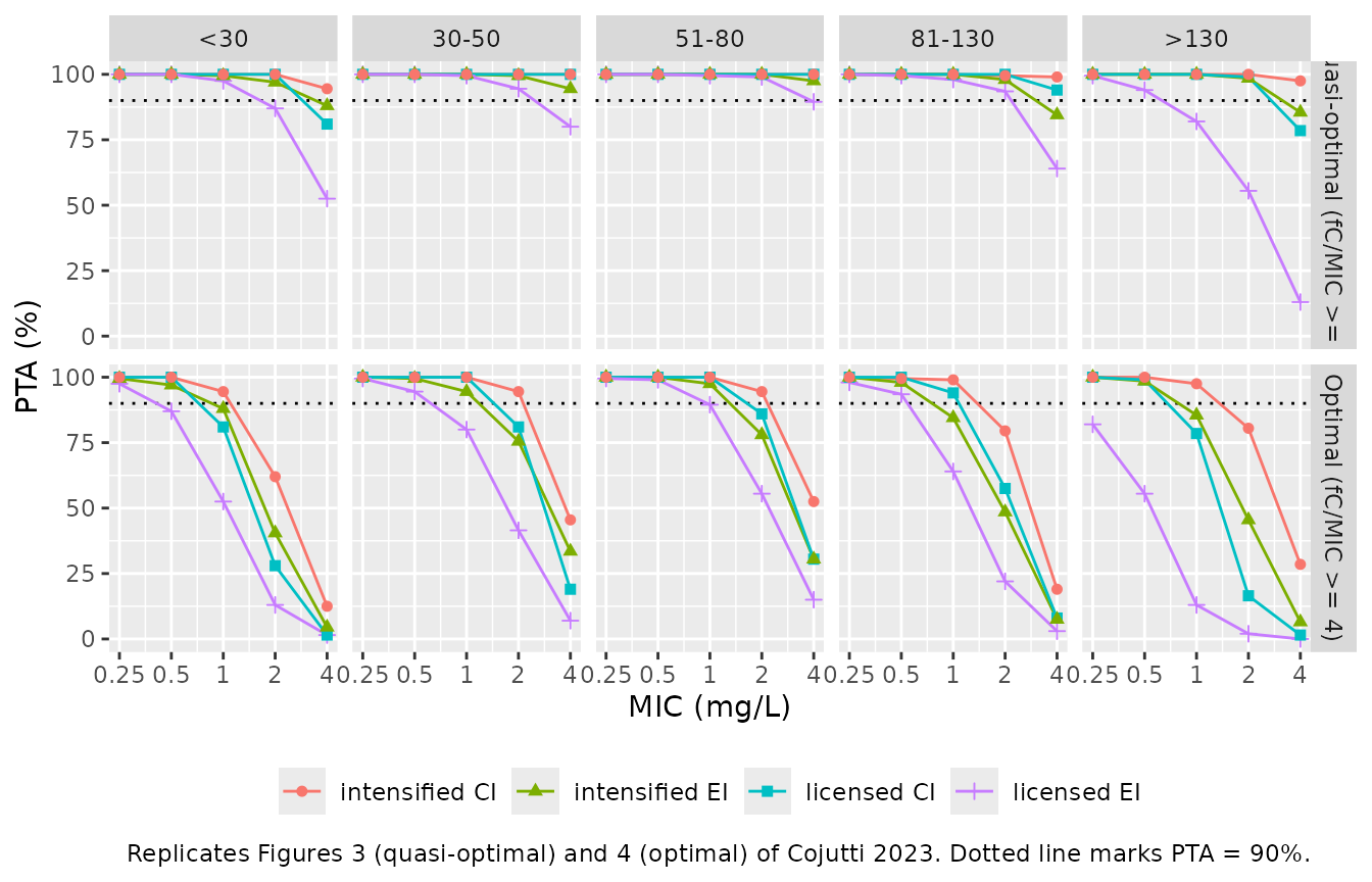
get_pta <- function(cls, lvl, md, tgt, mic_val) {
  v <- pta$pta[pta$class == cls & pta$level == lvl & pta$mode == md &
               pta$target == tgt & pta$mic == mic_val]
  stopifnot(length(v) == 1)
  v
}

classes <- c("<30", "30-50", "51-80", "81-130", ">130")

claims <- tibble::tibble(
  class = classes,
  # Results 3.3, optimal target, licensed CI: PTA >= 90% only up to MIC 1 mg/L
  # for eGFR 30-130, and only up to MIC 0.5 mg/L for eGFR <30 and >130.
  paper_ci_optimal_mic_cutoff = c(0.5, 1, 1, 1, 0.5),
  ci_mic0.5 = unname(vapply(classes, get_pta, 0, lvl = "licensed", md = "CI", tgt = 4, mic_val = 0.5)),
  ci_mic1   = unname(vapply(classes, get_pta, 0, lvl = "licensed", md = "CI", tgt = 4, mic_val = 1)),
  ci_mic2   = unname(vapply(classes, get_pta, 0, lvl = "licensed", md = "CI", tgt = 4, mic_val = 2))
) |>
  dplyr::mutate(
    sim_cutoff = dplyr::case_when(ci_mic2 >= 90 ~ 2, ci_mic1 >= 90 ~ 1,
                                  ci_mic0.5 >= 90 ~ 0.5, TRUE ~ 0.25),
    agrees = sim_cutoff == paper_ci_optimal_mic_cutoff
  )

claims |>
  dplyr::rename(
    "eGFR class"                = class,
    "Paper MIC cutoff (mg/L)"   = paper_ci_optimal_mic_cutoff,
    "PTA at MIC 0.5 (%)"        = ci_mic0.5,
    "PTA at MIC 1 (%)"          = ci_mic1,
    "PTA at MIC 2 (%)"          = ci_mic2,
    "Simulated MIC cutoff"      = sim_cutoff,
    "Agrees"                    = agrees
  ) |>
  knitr::kable(digits = 1,
               caption = paste("Licensed continuous infusion, optimal target (fCss/MIC >= 4).",
"Replicates the Results 3.3 statement on highest MIC attaining PTA >= 90%."))| eGFR class | Paper MIC cutoff (mg/L) | PTA at MIC 0.5 (%) | PTA at MIC 1 (%) | PTA at MIC 2 (%) | Simulated MIC cutoff | Agrees |
|---|---|---|---|---|---|---|
| <30 | 0.5 | 99.3 | 81.3 | 28.9 | 0.5 | TRUE |
| 30-50 | 1.0 | 100.0 | 98.5 | 71.4 | 1.0 | TRUE |
| 51-80 | 1.0 | 100.0 | 99.8 | 84.8 | 1.0 | TRUE |
| 81-130 | 1.0 | 100.0 | 96.7 | 56.7 | 1.0 | TRUE |
| >130 | 0.5 | 99.1 | 77.9 | 20.8 | 0.5 | TRUE |
All five renal classes reproduce the paper’s stated MIC cutoff exactly. The same check for the quasi-optimal target with extended infusion at the EUCAST S. aureus breakpoint of 2 mg/L:
ei_claims <- tibble::tibble(
  class = classes,
  # Results 3.3: at MIC 2 mg/L the quasi-optimal target is attained with the
  # licensed EI regimens in eGFR 30-130 only, and by CI at eGFR >130.
  paper_ei_attains = c(FALSE, TRUE, TRUE, TRUE, FALSE),
  ei_pta = unname(vapply(classes, get_pta, 0, lvl = "licensed", md = "EI", tgt = 1, mic_val = 2)),
  ci_pta = unname(vapply(classes, get_pta, 0, lvl = "licensed", md = "CI", tgt = 1, mic_val = 2))
) |>
  dplyr::mutate(sim_ei_attains = ei_pta >= 90, agrees = sim_ei_attains == paper_ei_attains)

ei_claims |>
  dplyr::rename(
    "eGFR class"              = class,
    "Paper: EI attains >=90%" = paper_ei_attains,
    "Simulated EI PTA (%)"    = ei_pta,
    "Simulated CI PTA (%)"    = ci_pta,
    "Simulated: EI attains"   = sim_ei_attains,
    "Agrees"                  = agrees
  ) |>
  knitr::kable(digits = 1,
               caption = paste("Licensed regimens at MIC 2 mg/L, quasi-optimal target",
"(fC/MIC >= 1). Replicates the Results 3.3 statement."))| eGFR class | Paper: EI attains >=90% | Simulated EI PTA (%) | Simulated CI PTA (%) | Simulated: EI attains | Agrees |
|---|---|---|---|---|---|
| <30 | FALSE | 87.9 | 99.3 | FALSE | TRUE |
| 30-50 | TRUE | 96.0 | 100.0 | TRUE | TRUE |
| 51-80 | TRUE | 99.0 | 100.0 | TRUE | TRUE |
| 81-130 | TRUE | 92.1 | 100.0 | TRUE | TRUE |
| >130 | FALSE | 59.3 | 99.1 | FALSE | TRUE |
stopifnot(
  all(ei_claims$agrees),
  # "... and by CI in that of eGFR > 130 mL/min/1.73 m^2"
  ei_claims$ci_pta[ei_claims$class == ">130"] >= 90
)
Both statements reproduce: extended infusion attains the quasi-optimal target at MIC 2 mg/L in the three intermediate renal classes but fails at eGFR < 30 and eGFR > 130, and continuous infusion rescues the augmented-renal-clearance class. Together with the optimal-target table above, eleven independent binary claims from Results 3.3 are reproduced.
The paper’s conclusion follows directly from the figure: against MRSA at the 2 mg/L breakpoint, the optimal target is not reached by any licensed regimen in the augmented-renal-clearance class, and intensified continuous infusion is required.
Assumptions and deviations
-
Covariate functional form. Results 3.2 describes
both covariates as “power function[s]”, but the reported eGFR
coefficient of 0.011 is irreconcilable with a power exponent (it would
make the effect negligible, contradicting the abstract and the paper’s
own median individual CL of 4.04 L/h). The model encodes the exponential
form
cl = exp(lcl) * exp(0.011 * CRCL), which reproduces the reported median to within 5.7%; see the “Covariate functional form” section for the full scoring against six candidate forms. Trusting the numbers over the prose follows the standing convention for text-vs-value conflicts. -
Uncentered eGFR. Following from the above,
exp(lcl) = 1.7 L/his the clearance extrapolated to eGFR = 0 and is not a typical value at any physiological renal function. This is consistent with the base-model CL of 3.43 L/h dropping to 1.7 L/h when the covariate enters. - Sex reference category. Table 2 reports a single “Gender on V1” coefficient of 0.39 without saying which sex is the reference. Female was identified as the reference by back-solving against the reported median individual V1 of 19.7 L; see the “Covariate functional form” section.
-
IIV scale. Table 2 reports IIV as “%CV”. The model
uses the standard log-normal identity
omega^2 = log(1 + CV^2). The alternative reading (that the paper printed100 * omega) is numerically indistinguishable for CL, Q2, V1, and V3, but for V2 it impliesomega = 2.681, which over-predicts the paper’s own reported individual V2 range of 7.6-526.0 L by roughly 85-fold;omega = 1.450over-predicts by only ~3.6-fold, consistent with empirical-Bayes shrinkage on a poorly identified peripheral volume. -
Residual error parameterization. Table 2 reports a
combined error model with
a = 1.44andb = 0.22but does not state whether Monolix’scombined1(sd = a + b*f) orcombined2(sd = sqrt(a^2 + (b*f)^2)) was used. The model file uses nlmixr2’sadd() + prop(), which iscombined2. This affects the residual-error magnitude only, not the structural model or any PTA result (target attainment is computed on model predictions). - Representative eGFR per renal class. The Monte Carlo in Methods 2.4 is stratified into five eGFR classes but the paper does not state the eGFR value or distribution used within each class. The class midpoints (20, 40, 65, 105, and 150 mL/min/1.73 m^2) are used here. All eleven of the paper’s binary PTA statements reproduce under this choice.
- Cumulative fraction of response (Table 3) is not reproduced. CFR requires the EUCAST MIC distributions for MRSA and MRSE, which the paper cites (its reference 20) but does not print. PTA by MIC, which is the model-dependent quantity, is reproduced instead.
- Cohort size. The paper ran 1000 Monte Carlo simulations per scenario; the vignette uses 5000 per arm so that PTA values carry a Monte Carlo standard error of at most 0.7 percentage points. The asserted claims are those where the simulated PTA is clear of the 90% threshold by more than three standard errors.
- Virtual cohort covariates. The eGFR distribution is a piecewise-linear interpolation through the Table 1 quartiles with tails set to 10 and 180 mL/min/1.73 m^2; the paper reports only the median and IQR. Subjects are placed at deterministic quantiles rather than drawn at random so the comparison against the observed concentrations is stable across runs.
- TDM-guided dose adjustment is not modelled. The observed-concentration comparison simulates the Methods 2.1 starting regimens held for one week, whereas the real cohort had doses adjusted by TDM. The median daily dose in Table 1 (1500 mg, IQR 1000-1500) matches the simulated starting regimens, so the comparison remains informative.
- Serum albumin unit label. Table 1 gives serum albumin as “3.1 (2.7-3.4) g/L”, which is a unit-label error in the source (these are g/dL values). Albumin was not among the screened covariates and is not used by the model.
-
Covariates screened but not retained. Age, weight,
and height were tested (Methods 2.3) but did not enter the final model;
they are recorded in the model file’s
covariatesDataExcludedmetadata. In particular the model applies no allometric weight scaling.