Remimazolam (Chen 2025)
Source:vignettes/articles/Chen_2025_remimazolam.Rmd
Chen_2025_remimazolam.RmdModel and source
- Citation: Chen J, Wang X, Chen D, Liu X, Peng K, Tang R, Hu L, Wang Y, Bai Y, Chang L, Chen C. (2025). Population pharmacokinetic analysis of remimazolam after continuous infusion for sedation in critically ill patients. Front Pharmacol 16:1526266. doi:10.3389/fphar.2025.1526266.
- Description: Two-compartment population pharmacokinetic model for remimazolam given by continuous intravenous infusion for sedation in critically ill adults in the intensive care unit (Chen 2025). This is the first published popPK analysis of remimazolam in an ICU population, and the study’s central finding is a negative one: of the 27 candidate covariates screened – including body weight, age, sex, hepatic and renal function markers, and the presence of extracorporeal membrane oxygenation (ECMO) or continuous renal replacement therapy (CRRT) – none survived backward elimination, so the final model carries no covariate effects at all. Disposition is described by first-order elimination from a central compartment plus a single peripheral compartment; inter-individual variability is exponential on all four structural parameters and residual error is purely proportional. The authors’ companion Monte Carlo simulation shows that the context-sensitive half-time is essentially independent of infusion duration (15.6-21 min over infusions from 0.5 to 72 h), which is the property that makes the drug attractive for long-term ICU sedation. Note that the authors chose a two-compartment structure where most prior remimazolam analyses used three compartments; they attribute this to sparse arterial sampling confined to the post-infusion elimination phase (see the validation vignette).
- Article: https://doi.org/10.3389/fphar.2025.1526266
- Supplement: https://www.frontiersin.org/articles/10.3389/fphar.2025.1526266/full#supplementary-material
Population
Chen 2025 is a prospective, single-centre observational study run at Maoming People’s Hospital (Guangdong, China) between April and December 2022. Thirty-two critically ill adults (24 men, 8 women) who were receiving remimazolam besylate by continuous micropump infusion for ICU sedation contributed 236 analysable plasma concentrations out of 243 collected; seven were discarded as implausibly high or low (Section 3.1). Median age was 62 years (range 26-79), median weight 63 kg (47-98 kg) and median BMI 22.67 kg/m2 (Table 1).
The cohort is genuinely critically ill rather than merely hospitalised: the median APACHE II score was 26 (range 15-41) and in-hospital mortality was 25%. Admission diagnoses were respiratory failure (28.7%), heart failure (26.0%), severe pneumonia (15.1%), septic shock (12.3%), acute myocardial infarction (11.0%) and COPD (6.8%). Organ function spanned normal to severely impaired (ALT 7.8-549.2 U/L; creatinine clearance 8.69-193.83 mL/min). Eighteen of the 32 patients were supported with ECMO and 14 were on CRRT. Nearly all (96.8%) also received remifentanil for analgesia.
Dosing was pragmatic rather than protocolised: the bedside clinician titrated the micropump to the target Richmond Agitation-Sedation Scale score, giving 2-17.28 mg/h (median 6 mg/h) for 6.15-294.9 h (median 8.33 h). No loading dose was part of the observational protocol. Arterial samples were drawn at the moment the infusion was stopped and at 10, 20, 30, 60, 90, 120 and 240 min afterwards, so the design informs the post-infusion disposition phase and essentially nothing else – a point that matters for interpreting the structural model (see Assumptions and deviations).
The same information is available programmatically via the model’s
population metadata
(readModelDb("Chen_2025_remimazolam")()$population).
Source trace
Per-parameter origin is recorded as an in-file comment next to each
ini() entry in
inst/modeldb/specificDrugs/Chen_2025_remimazolam.R.
Collected here for review.
| Equation / parameter | Value | Source location |
|---|---|---|
lcl (CL) |
58.2 L/h | Table 2, Estimate column (RSE 10.6%) |
lvc (V1) |
25.5 L | Table 2, Estimate column (RSE 12.8%) |
lq (Q) |
20.0 L/h | Table 2, Estimate column (RSE 21.8%) |
lvp (V2) |
34.5 L | Table 2, Estimate column (RSE 17.0%) |
etalcl |
0.503^2 | Table 2: IIV-CL = 50.3% (RSE 15.6%, shrinkage 1%) |
etalvc |
0.165^2 | Table 2: IIV-V1 = 16.5% (RSE 68.7%, shrinkage 69%) |
etalq |
0.657^2 | Table 2: IIV-Q = 65.7% (RSE 50.0%, shrinkage 27%) |
etalvp |
0.612^2 | Table 2: IIV-V2 = 61.2% (RSE 24.7%, shrinkage 15%) |
propSd |
0.25 | Table 2: proportional error 25.0% (RSE 13.0%); Section 3.2 |
| Two-compartment structure | n/a | Section 3.2; Supplementary Table S2 (1- vs 2- vs 3-compartment) |
kel, k12, k21
|
derived | Supplementary Table S4 (k10 2.28, k12 0.78, k21 0.58 /h) |
| Exponential IIV, proportional RUV | n/a | Section 2.4 |
Cc unit conversion (x1000) |
n/a | Section 2.3: assay reports ng/mL over 1.0-1000 ng/mL |
| Covariate screen (none retained) | n/a | Section 3.2; Supplementary Table S3 (54 runs) |
Six screened covariates have no canonical entry in the covariate
register and were deliberately not given invented names in the model
file, since none carries a point estimate and none appears in
model(): ECMO status (Supplementary Table S3 runs 11-12),
serum uric acid (25-26), CKD-EPI eGFR (29-30), procalcitonin (33-34),
arterial pH (41-42) and platelet count (43-44). The remaining 21
screened covariates are documented under
covariatesDataExcluded in the model file.
Closed-form check against Supplementary Table S4
Chen 2025 publishes the derived micro-constants and hybrid half-lives
separately from the primary parameters, which gives an exact arithmetic
gate on the transcription: the packaged ini() values must
reproduce Supplementary Table S4 without any fitting.
mod <- readModelDb("Chen_2025_remimazolam")
ui  <- rxode2::rxode(mod)
#> ℹ parameter labels from comments will be replaced by 'label()'

theta <- setNames(ui$theta, names(ui$theta))
CL <- exp(theta[["lcl"]]); V1 <- exp(theta[["lvc"]])
Q  <- exp(theta[["lq"]]);  V2 <- exp(theta[["lvp"]])

k10 <- CL / V1
k12 <- Q  / V1
k21 <- Q  / V2

# Hybrid rate constants of the two-compartment system.
s     <- k10 + k12 + k21
alpha <- (s + sqrt(s^2 - 4 * k10 * k21)) / 2
beta  <- (s - sqrt(s^2 - 4 * k10 * k21)) / 2

closed_form <- tibble::tribble(
  ~quantity,          ~model,          ~published, ~source,
  "k10 (1/h)",        k10,             2.28,       "Suppl. Table S4",
  "k12 (1/h)",        k12,             0.78,       "Suppl. Table S4",
  "k21 (1/h)",        k21,             0.58,       "Suppl. Table S4",
  "t1/2 alpha (h)",   log(2) / alpha,  0.21,       "Suppl. Table S4",
  "t1/2 beta (h)",    log(2) / beta,   1.70,       "Suppl. Table S4",
  "Vss = V1+V2 (L)",  V1 + V2,         60.0,       "Table 2 (V1 + V2)"
) |>
  mutate(`difference (%)` = 100 * (model - published) / published)

closed_form |>
  dplyr::rename(
    "Quantity"      = quantity,
    "Model"         = model,
    "Published"     = published,
    "Source"        = source
  ) |>
  knitr::kable(digits = 3,
caption = "Derived quantities vs Chen 2025 Supplementary Table S4.")| Quantity | Model | Published | Source | difference (%) |
|---|---|---|---|---|
| k10 (1/h) | 2.282 | 2.28 | Suppl. Table S4 | 0.103 |
| k12 (1/h) | 0.784 | 0.78 | Suppl. Table S4 | 0.553 |
| k21 (1/h) | 0.580 | 0.58 | Suppl. Table S4 | -0.050 |
| t1/2 alpha (h) | 0.214 | 0.21 | Suppl. Table S4 | 1.945 |
| t1/2 beta (h) | 1.696 | 1.70 | Suppl. Table S4 | -0.225 |
| Vss = V1+V2 (L) | 60.000 | 60.00 | Table 2 (V1 + V2) | 0.000 |
# The published values are rounded to 2 significant figures, so the model must
# agree exactly once rounded the same way.
stopifnot(
  round(k10, 2)          == 2.28,
  round(k12, 2)          == 0.78,
  round(k21, 2)          == 0.58,
  round(log(2) / alpha, 2) == 0.21,
  round(log(2) / beta, 1)  == 1.7,
  V1 + V2                == 60.0
)
This also settles a genuine ambiguity in the paper. The Abstract and
Section 3.2 quote Q as 21.9 L/h, but Table 2’s Estimate
column gives 20.0 L/h and lists 21.9 as the bootstrap
median. Only 20.0 reproduces the published micro-constants:
20.0/25.5 = 0.784 and 20.0/34.5 = 0.580 versus
the printed 0.78 and 0.58, whereas 21.9 would give 0.859 and 0.635. The
model therefore uses 20.0 L/h.
tibble::tibble(
  `Q reading`   = c("20.0 L/h (Table 2 estimate)", "21.9 L/h (Table 2 bootstrap median)"),
  `implied k12` = c(20.0 / V1, 21.9 / V1),
  `implied k21` = c(20.0 / V2, 21.9 / V2)
) |>
  mutate(`matches S4 (0.78 / 0.58)?` =
           ifelse(round(`implied k12`, 2) == 0.78 & round(`implied k21`, 2) == 0.58,
                  "yes", "no")) |>
knitr::kable(digits = 3, caption = "Which reported Q reproduces Supplementary Table S4.")| Q reading | implied k12 | implied k21 | matches S4 (0.78 / 0.58)? |
|---|---|---|---|
| 20.0 L/h (Table 2 estimate) | 0.784 | 0.580 | yes |
| 21.9 L/h (Table 2 bootstrap median) | 0.859 | 0.635 | no |
Virtual cohort
Original observed data are not publicly available. The simulations below use virtual populations dosed according to the regimens Chen 2025 itself simulated (Section 2.6). The model carries no covariates, so a “cohort” here is defined entirely by its dosing regimen; between-subject differences come from the four exponential IIV terms.
set.seed(20250709)

N_PER_ARM <- 200L  # cap per the nlmixr2lib validation convention

# One arm = a 1-min loading dose followed by a constant-rate maintenance
# infusion, then washout. Times in hours, amounts in mg, rates in mg/h.
make_arm <- function(n, load_mg, maint_mg_h, maint_h, washout_h,
                     arm, id_offset = 0L, obs_grid = NULL) {
  ids <- id_offset + seq_len(n)
  load_h <- 1 / 60

  dosing <- dplyr::bind_rows(
    if (load_mg > 0) {
      tidyr::expand_grid(id = ids, time = 0) |>
        dplyr::mutate(amt = load_mg, rate = load_mg / load_h, evid = 1L)
    },
    tidyr::expand_grid(id = ids, time = load_h) |>
      dplyr::mutate(amt = maint_mg_h * maint_h, rate = maint_mg_h, evid = 1L)
  ) |>
    dplyr::mutate(cmt = "central")

  if (is.null(obs_grid)) {
    obs_grid <- sort(unique(c(
      seq(0, maint_h + washout_h, by = 0.05),
      maint_h + c(10, 20, 30, 60, 90, 120, 240) / 60  # Chen 2025 sampling times
    )))
  }
  obs <- tidyr::expand_grid(id = ids, time = obs_grid) |>
    dplyr::mutate(amt = NA_real_, rate = NA_real_, evid = 0L,
                  # cmt is the ODE STATE, never the observable name "Cc"
                  cmt = "central")

  dplyr::bind_rows(dosing, obs) |>
    dplyr::mutate(arm = arm) |>
    dplyr::arrange(id, time, dplyr::desc(evid))
}
Replicate published figures
Figures 7A and 7B – concentration-time curves under the simulated dose scenarios
Chen 2025 Section 2.6 simulated loading doses of 3-8 mg given over 1 min followed by maintenance infusions of 6-18 mg/h for up to 16 h. Section 3.3 reports that the concentration “rapidly peaked” after the loading dose and then “tended towards a steady-state”, reaching steady state in about 4 h. These are population predictions, so they are reproduced with the random effects zeroed.
scenarios <- tibble::tribble(
  ~arm,                    ~load_mg, ~maint_mg_h,
  "3 mg load, 6 mg/h",     3,        6,
  "5 mg load, 10 mg/h",    5,        10,
  "6.5 mg load, 14 mg/h",  6.5,      14,
  "8 mg load, 18 mg/h",    8,        18
)

ev_typ <- dplyr::bind_rows(
  lapply(seq_len(nrow(scenarios)), function(i) {
    make_arm(n = 1L,
             load_mg    = scenarios$load_mg[i],
             maint_mg_h = scenarios$maint_mg_h[i],
             maint_h    = 16, washout_h = 4,
             arm        = scenarios$arm[i],
             id_offset  = (i - 1L) * 1L,
             obs_grid   = seq(0, 20, by = 1 / 120))
  })
)
stopifnot(!anyDuplicated(ev_typ[ev_typ$evid == 0L, c("id", "time")]))

mod_typ <- rxode2::zeroRe(mod)
#> ℹ parameter labels from comments will be replaced by 'label()'
sim_typ <- rxode2::rxSolve(mod_typ, events = ev_typ, keep = "arm") |>
  as.data.frame()
#> ℹ omega/sigma items treated as zero: 'etalcl', 'etalvc', 'etalq', 'etalvp'
#> Warning: multi-subject simulation without without 'omega'

sim_typ$arm <- factor(sim_typ$arm, levels = scenarios$arm)

ggplot(sim_typ, aes(time, Cc, colour = arm)) +
  geom_line(linewidth = 0.8) +
  geom_vline(xintercept = 16, linetype = "dashed", colour = "grey40") +
  labs(x = "Time (h)", y = "Remimazolam plasma concentration (ng/mL)",
       colour = "Regimen",
       title = "Figures 7A / 7B - loading plus maintenance infusion scenarios",
       caption = paste("Replicates Figures 7A and 7B of Chen 2025.",
                       "Dashed line = end of the 16 h maintenance infusion.")) +
  theme_bw()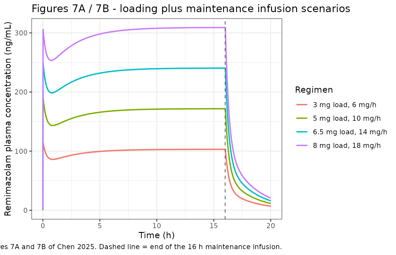
The steady-state concentration of a constant-rate infusion is
R/CL, and the approach to it is governed by the terminal
half-life. Both are checked directly.
# rxSolve returns observation records only, so there is no evid column here.
ss_check <- sim_typ |>
  dplyr::group_by(arm) |>
  dplyr::summarise(
    `C at 4 h (ng/mL)`  = Cc[which.min(abs(time - 4))],
    `C at 16 h (ng/mL)` = Cc[which.min(abs(time - 16))],
    .groups = "drop"
  ) |>
  dplyr::mutate(arm = as.character(arm)) |>
  dplyr::left_join(scenarios, by = "arm") |>
  dplyr::mutate(`Css analytic (ng/mL)`    = 1000 * maint_mg_h / CL,
                `fraction of Css at 4 h`  = `C at 4 h (ng/mL)` / `Css analytic (ng/mL)`,
                `fraction of Css at 16 h` = `C at 16 h (ng/mL)` / `Css analytic (ng/mL)`) |>
  dplyr::select(-load_mg, -maint_mg_h)
stopifnot(nrow(ss_check) == nrow(scenarios), !anyNA(ss_check$`Css analytic (ng/mL)`))

knitr::kable(ss_check, digits = 3,
caption = "Approach to steady state; Chen 2025 Section 3.3 reports about 4 h.")| arm | C at 4 h (ng/mL) | C at 16 h (ng/mL) | Css analytic (ng/mL) | fraction of Css at 4 h | fraction of Css at 16 h |
|---|---|---|---|---|---|
| 3 mg load, 6 mg/h | 97.649 | 103.052 | 103.093 | 0.947 | 1 |
| 5 mg load, 10 mg/h | 162.748 | 171.754 | 171.821 | 0.947 | 1 |
| 6.5 mg load, 14 mg/h | 227.615 | 240.454 | 240.550 | 0.946 | 1 |
| 8 mg load, 18 mg/h | 292.482 | 309.154 | 309.278 | 0.946 | 1 |
# Chen 2025 Section 3.3: "it took about 4 h to achieve steady state".
# 4 h is ~2.4 terminal half-lives, so the model must be within a few percent
# of Css by then and essentially at Css by the end of the 16 h infusion.
stopifnot(
  all(ss_check$`fraction of Css at 4 h`  > 0.90),
  all(ss_check$`fraction of Css at 16 h` > 0.99),
  all(ss_check$`fraction of Css at 16 h` <= 1.0)
)
At the most commonly administered ICU rate in this cohort (6 mg/h, Table 1) the model predicts a steady-state concentration of 103 ng/mL. This independently reproduces the observation in Section 4.3 that routine ICU dosing did not reach the 400-1200 ng/mL sedation range reported for remimazolam monotherapy – the authors attribute the adequate sedation seen at these lower concentrations to co-administered remifentanil in 96.8% of patients.
stopifnot(1000 * 6 / CL < 400) # Section 4.3: routine dosing falls short of 400-1200 ng/mLFigure 7C – context-sensitive decrement times
Chen 2025 simulated the time required for a 10% to 90% decrement in plasma concentration after stopping a 12 mg/h maintenance infusion of 0.5 to 72 h (Section 2.6), and reports the 50% decrement – the context-sensitive half-time (CSHT) – as 15.6, 18 and 21 min after 0.5, 2 and 8 h of infusion, plateauing thereafter (Section 3.3). CSDTs were computed “from population predicted values”, so the typical-value model is the right basis.
# Time for the concentration to fall to `keep_frac` of its value at infusion
# stop, after a constant-rate infusion of `dur_h` hours.
decrement_time <- function(dur_h, decrements, rate_mg_h = 12) {
  post <- c(seq(0, 1, by = 1 / 600), seq(1.01, 36, by = 0.01))  # 6 s then 36 s resolution
  ev <- dplyr::bind_rows(
    tibble::tibble(id = 1L, time = 0, amt = rate_mg_h * dur_h,
                   rate = rate_mg_h, evid = 1L, cmt = "central"),
    tibble::tibble(id = 1L, time = dur_h + post, amt = NA_real_,
                   rate = NA_real_, evid = 0L, cmt = "central")
  )
  out <- rxode2::rxSolve(mod_typ, events = ev) |> as.data.frame()
  out <- out[out$time >= dur_h, ]   # rxSolve returns observation rows only
  cstop <- out$Cc[which.min(abs(out$time - dur_h))]
  stopifnot(cstop > 0, nrow(out) > 100)

  vapply(decrements, function(d) {
    idx <- which(out$Cc <= (1 - d) * cstop)[1]
    if (is.na(idx)) NA_real_ else (out$time[idx] - dur_h) * 60  # minutes
  }, numeric(1))
}

decrements <- seq(0.1, 0.9, by = 0.1)
durations  <- c(0.5, 1, 2, 4, 8, 12, 24, 48, 72)

csdt <- tidyr::expand_grid(duration_h = durations, decrement = decrements) |>
  dplyr::mutate(minutes = NA_real_)
for (d in durations) {
  csdt$minutes[csdt$duration_h == d] <- decrement_time(d, decrements)
}
#> ℹ omega/sigma items treated as zero: 'etalcl', 'etalvc', 'etalq', 'etalvp'
#> ℹ omega/sigma items treated as zero: 'etalcl', 'etalvc', 'etalq', 'etalvp'
#> ℹ omega/sigma items treated as zero: 'etalcl', 'etalvc', 'etalq', 'etalvp'
#> ℹ omega/sigma items treated as zero: 'etalcl', 'etalvc', 'etalq', 'etalvp'
#> ℹ omega/sigma items treated as zero: 'etalcl', 'etalvc', 'etalq', 'etalvp'
#> ℹ omega/sigma items treated as zero: 'etalcl', 'etalvc', 'etalq', 'etalvp'
#> ℹ omega/sigma items treated as zero: 'etalcl', 'etalvc', 'etalq', 'etalvp'
#> ℹ omega/sigma items treated as zero: 'etalcl', 'etalvc', 'etalq', 'etalvp'
#> ℹ omega/sigma items treated as zero: 'etalcl', 'etalvc', 'etalq', 'etalvp'
stopifnot(!anyNA(csdt$minutes))

ggplot(csdt, aes(duration_h, minutes, colour = factor(100 * decrement))) +
  geom_line(linewidth = 0.7) +
  geom_point(size = 1) +
  scale_x_log10(breaks = durations, labels = durations) +
  labs(x = "Infusion duration (h, log scale)",
       y = "Decrement time (min)",
       colour = "Decrement (%)",
       title = "Figure 7C - context-sensitive decrement times, 12 mg/h infusion",
       caption = "Replicates Figure 7C of Chen 2025.") +
  theme_bw()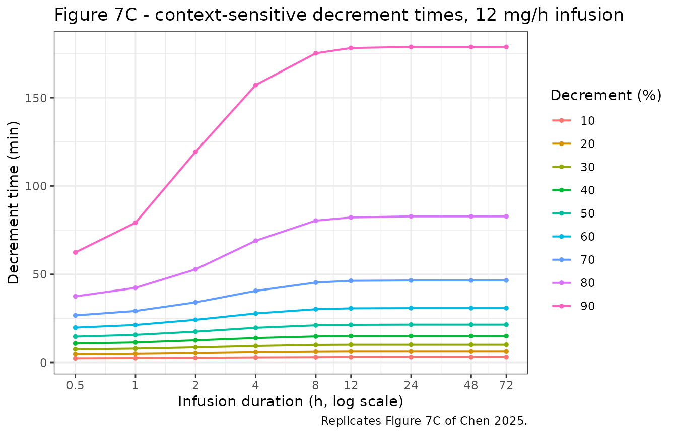
csht <- csdt |> dplyr::filter(decrement == 0.5)

csht_cmp <- csht |>
  dplyr::filter(duration_h %in% c(0.5, 2, 8)) |>
  dplyr::transmute(`Infusion duration (h)` = duration_h,
                   `Model CSHT (min)`      = minutes,
                   `Chen 2025 (min)`       = c(15.6, 18, 21)) |>
  dplyr::mutate(`difference (min)` = `Model CSHT (min)` - `Chen 2025 (min)`,
                `difference (%)`   = 100 * `difference (min)` / `Chen 2025 (min)`)

knitr::kable(csht_cmp, digits = 2,
caption = "Context-sensitive half-time vs Chen 2025 Section 3.3.")| Infusion duration (h) | Model CSHT (min) | Chen 2025 (min) | difference (min) | difference (%) |
|---|---|---|---|---|
| 0.5 | 14.7 | 15.6 | -0.9 | -5.77 |
| 2.0 | 17.5 | 18.0 | -0.5 | -2.78 |
| 8.0 | 21.1 | 21.0 | 0.1 | 0.48 |
# Chen 2025 computed CSDTs by Monte Carlo over 1,000 subjects while this is a
# typical-value profile, so exact agreement is not expected; agreement to
# within 1 min is.
stopifnot(all(abs(csht_cmp$`difference (min)`) < 1))

# Section 3.3 / 4.2: "all curves plateaued after 24 h" and the CSHT is
# "independent of prolonged infusion", ranging over 15.6-21 min.
plateau <- csht$minutes[csht$duration_h >= 24]
stopifnot(
  diff(range(plateau)) < 0.5,                       # flat beyond 24 h
  max(csht$minutes) - min(csht$minutes) < 8,        # whole range is narrow
  all(csht$minutes >= 14), all(csht$minutes <= 22)  # brackets the published 15.6-21
)
The model reproduces the paper’s headline pharmacological claim: the CSHT rises only from 14.7 min after a 30-min infusion to 21.5 min after 72 h, i.e. remimazolam does not accumulate in a way that delays recovery. Note that the 90% decrement time does keep growing with infusion duration – it is the clinically relevant 10-50% decrements that plateau.
PKNCA validation
Chen 2025 reports no NCA table, but Supplementary Table S4 publishes a terminal half-life of 1.7 h (95% CI 0.83-4.3), which NCA can be checked against. Three arms spanning the simulated maintenance range are run with full between-subject variability.
Chen 2025’s own sampling stopped 240 min after the infusion, which is only about 2.4 terminal half-lives, so it is worth checking whether that window is long enough to recover the terminal slope at all. Both are therefore run: the paper’s actual 4 h window and an extended 12 h window.
nca_arms <- tibble::tribble(
  ~arm,       ~maint_mg_h,
  "6 mg/h",   6,
  "12 mg/h",  12,
  "18 mg/h",  18
)

MAINT_H <- 8  # close to the cohort median infusion duration of 8.33 h

events <- dplyr::bind_rows(
  lapply(seq_len(nrow(nca_arms)), function(i) {
    make_arm(n = N_PER_ARM, load_mg = 0,
             maint_mg_h = nca_arms$maint_mg_h[i],
             maint_h = MAINT_H, washout_h = 12,
             arm = nca_arms$arm[i],
             id_offset = (i - 1L) * N_PER_ARM,
             obs_grid = sort(unique(c(seq(0, MAINT_H, by = 0.25),
                                      MAINT_H + c(seq(0, 2, by = 1 / 60),
                                                  seq(2.25, 12, by = 0.25))))))
  })
)
stopifnot(!anyDuplicated(events[events$evid == 0L, c("id", "time")]))

sim <- rxode2::rxSolve(mod, events = events, keep = "arm") |> as.data.frame()
#> ℹ parameter labels from comments will be replaced by 'label()'

# Chen 2025 Section 2.3: the HPLC-MS/MS assay is linear over 1.0-1000 ng/mL, so
# 1.0 ng/mL is the lower limit of quantification. Subjects drawn from the tails
# of the (large) IIV distributions decay to the solver floor well before the end
# of the 12 h window; those records are orders of magnitude below anything the
# study could have measured, so the NCA below censors them exactly as the
# bioanalysis would. Guard that they are numerically negligible rather than a
# real negative excursion.
LLOQ <- 1.0
stopifnot(!anyNA(sim$Cc), min(sim$Cc) > -1e-6)
# Chen 2025 Figure 2 shows the post-infusion decline of every patient. This is
# the model's equivalent: the simulated post-stop decay by dose arm.
sim |>
  dplyr::filter(time >= MAINT_H, Cc >= LLOQ) |>
  dplyr::mutate(tad = time - MAINT_H) |>
  dplyr::group_by(arm, tad) |>
  dplyr::summarise(Q05 = quantile(Cc, 0.05), Q50 = median(Cc),
                   Q95 = quantile(Cc, 0.95), .groups = "drop") |>
  ggplot(aes(tad, Q50, colour = arm, fill = arm)) +
  geom_ribbon(aes(ymin = Q05, ymax = Q95), alpha = 0.2, colour = NA) +
  geom_line(linewidth = 0.8) +
  scale_y_log10() +
  labs(x = "Time after stopping the infusion (h)",
       y = "Remimazolam plasma concentration (ng/mL)",
       colour = "Maintenance rate", fill = "Maintenance rate",
       title = "Post-infusion decline (median with 5th-95th percentiles)",
       caption = paste("Model analogue of Figure 2 of Chen 2025, which plots the",
                       "observed post-infusion profiles. Records below the",
                       "1.0 ng/mL assay LLOQ are censored.")) +
  theme_bw()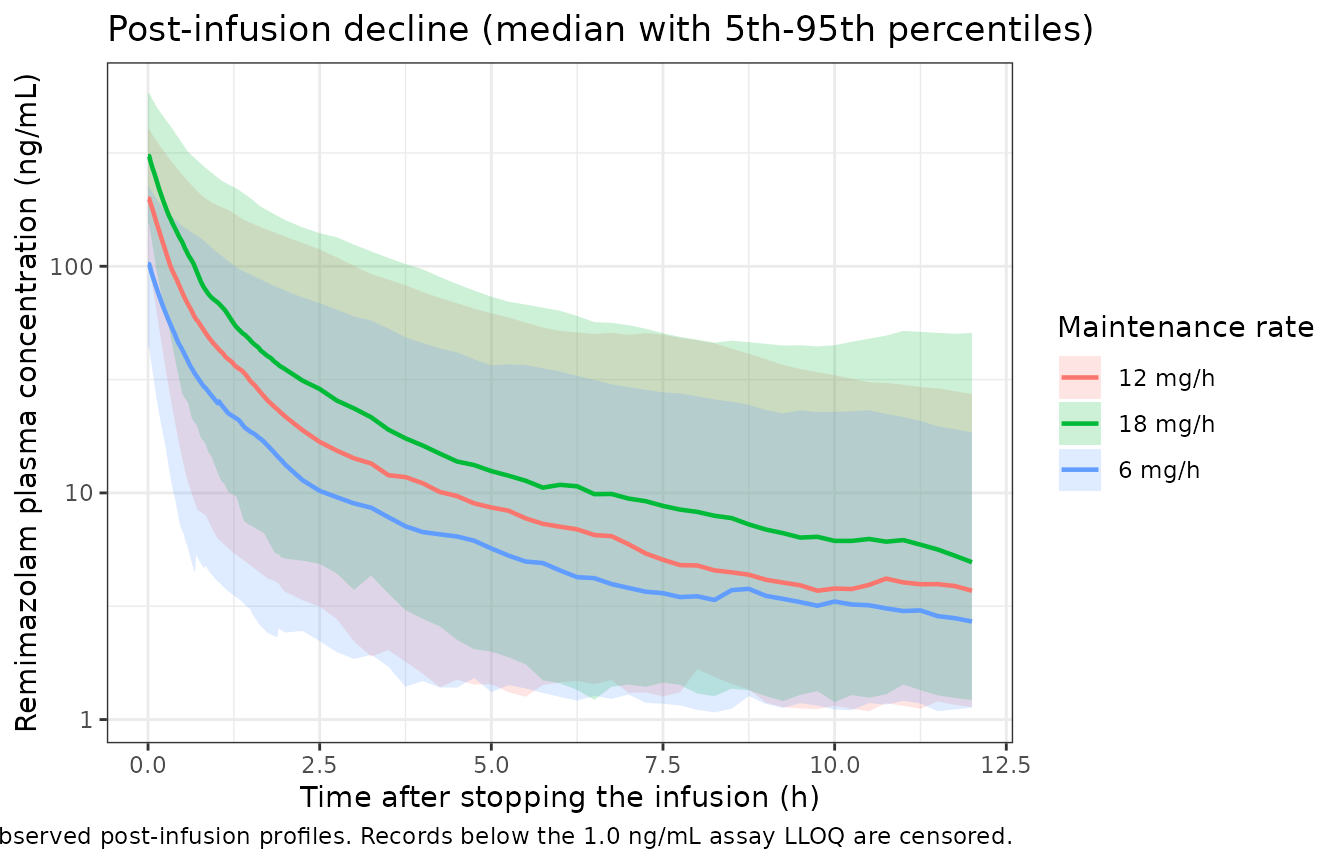
run_nca <- function(window_h) {
  sim_nca <- sim |>
    dplyr::filter(time <= MAINT_H + window_h) |>
    dplyr::filter(!is.na(Cc), Cc >= LLOQ) |>   # BLQ censoring at the 1.0 ng/mL assay limit
    dplyr::select(id, time, Cc, arm)

  # The LLOQ filter above removes the pre-dose record along with the BLQ tail,
  # so the time = 0 anchor PKNCA needs for AUC is restored explicitly here. The
  # infusion starts at t = 0, so the pre-dose concentration is 0.
  sim_nca <- dplyr::bind_rows(
    sim_nca,
    sim_nca |> dplyr::distinct(id, arm) |> dplyr::mutate(time = 0, Cc = 0)
  ) |>
    dplyr::distinct(id, arm, time, .keep_all = TRUE) |>
    dplyr::arrange(id, time)

  conc_obj <- PKNCA::PKNCAconc(sim_nca, Cc ~ time | arm + id)

  dose_df <- events |>
    dplyr::filter(evid == 1) |>
    dplyr::select(id, time, amt, arm)
  dose_obj <- PKNCA::PKNCAdose(dose_df, amt ~ time | arm + id,
                               route = "intravascular", duration = MAINT_H)

  intervals <- data.frame(start = 0, end = Inf,
                          cmax = TRUE, tmax = TRUE,
                          auclast = TRUE, half.life = TRUE)

  PKNCA::pk.nca(PKNCA::PKNCAdata(conc_obj, dose_obj, intervals = intervals))
}

nca_short <- run_nca(4)    # Chen 2025's actual sampling window
nca_long  <- run_nca(12)   # extended, resolves the terminal phase
published <- nca_arms |>
  dplyr::transmute(arm, half.life = 1.7)  # Suppl. Table S4, t1/2 beta

cmp_long <- nlmixr2lib::ncaComparisonTable(
  simulated = nca_long,
  reference = published,
  by        = "arm",
  units     = c(cmax = "ng/mL", tmax = "h", auclast = "ng*h/mL", half.life = "h"),
  tolerance_pct = 20
)

knitr::kable(cmp_long, digits = 3,
             caption = paste("Simulated NCA (12 h post-infusion window) vs Chen 2025",
"Supplementary Table S4. * differs from reference by >20%."))| NCA parameter | arm | Reference | Simulated | % diff |
|---|---|---|---|---|
| t½ (h) | 6 mg/h | 1.7 | 1.94 | +13.9% |
| t½ (h) | 12 mg/h | 1.7 | 1.81 | +6.3% |
| t½ (h) | 18 mg/h | 1.7 | 1.93 | +13.6% |
The strict gate on the half-life belongs on the
typical-value profile, not on the cohort median:
t1/2 beta is a non-linear function of all four structural
parameters, so with IIV this large the median of the individual
half-lives is not the half-life of the typical subject. The
typical-value NCA is therefore compared directly against the analytic
log(2)/beta.
ev_typ_nca <- make_arm(n = 1L, load_mg = 0, maint_mg_h = 12,
                       maint_h = MAINT_H, washout_h = 12, arm = "typical",
                       obs_grid = sort(unique(c(seq(0, MAINT_H, by = 0.25),
                                                MAINT_H + c(seq(0, 2, by = 1 / 60),
                                                            seq(2.25, 12, by = 0.25))))))
sim_typ_nca <- rxode2::rxSolve(mod_typ, events = ev_typ_nca) |> as.data.frame()
#> ℹ omega/sigma items treated as zero: 'etalcl', 'etalvc', 'etalq', 'etalvp'
if (is.null(sim_typ_nca$id)) sim_typ_nca$id <- 1L   # rxSolve drops `id` for a single subject

nca_typical_hl <- function(window_h) {
  d <- sim_typ_nca |>
    dplyr::filter(time <= MAINT_H + window_h, !is.na(Cc), Cc >= LLOQ) |>
    dplyr::select(id, time, Cc)
  d <- dplyr::bind_rows(d, tibble::tibble(id = 1L, time = 0, Cc = 0)) |>
    dplyr::distinct(id, time, .keep_all = TRUE) |>
    dplyr::arrange(time)
  res <- PKNCA::pk.nca(PKNCA::PKNCAdata(
    PKNCA::PKNCAconc(d, Cc ~ time | id),
    PKNCA::PKNCAdose(tibble::tibble(id = 1L, time = 0, amt = 12 * MAINT_H),
                     amt ~ time | id, route = "intravascular", duration = MAINT_H),
    intervals = data.frame(start = 0, end = Inf, half.life = TRUE)))
  as.data.frame(res) |>
    dplyr::filter(PPTESTCD == "half.life") |>
    dplyr::pull(PPORRES)
}

analytic_t_half <- log(2) / beta
typ_hl <- vapply(c(4, 12), nca_typical_hl, numeric(1))

tibble::tibble(
  `Sampling window`          = c("4 h (Chen 2025 protocol)", "12 h (extended)"),
  `Typical-value NCA t1/2 (h)` = typ_hl,
  `Analytic log(2)/beta (h)`   = analytic_t_half,
  `Published t1/2 beta (h)`    = 1.7
) |>
  dplyr::mutate(`vs analytic (%)`  = 100 * (`Typical-value NCA t1/2 (h)` - analytic_t_half) / analytic_t_half,
                `vs published (%)` = 100 * (`Typical-value NCA t1/2 (h)` - 1.7) / 1.7) |>
  knitr::kable(digits = 3,
caption = "Typical-value terminal half-life vs Chen 2025 Supplementary Table S4.")| Sampling window | Typical-value NCA t1/2 (h) | Analytic log(2)/beta (h) | Published t1/2 beta (h) | vs analytic (%) | vs published (%) |
|---|---|---|---|---|---|
| 4 h (Chen 2025 protocol) | 1.667 | 1.696 | 1.7 | -1.704 | -1.925 |
| 12 h (extended) | 1.681 | 1.696 | 1.7 | -0.882 | -1.105 |
# Both windows recover the analytic terminal half-life to within 2%, and the
# published 1.7 h to within 2.5%. Tightened to the accuracy actually achieved so
# that a future regression in the disposition parameters trips this gate.
stopifnot(
  all(abs(typ_hl - analytic_t_half) / analytic_t_half < 0.02),
  all(abs(typ_hl - 1.7) / 1.7 < 0.025)
)
The distribution half-life is only 0.21 h, so once records below the
assay LLOQ are censored, even the paper’s own 4 h post-infusion window
contains enough genuinely terminal points to recover
t1/2 beta; the extended window adds precision but does not
change the answer. The cohort medians are reported below for context,
and sit above the typical value as expected for a non-linear function of
log-normal inputs.
hl <- function(res, label) {
  as.data.frame(res) |>
    dplyr::filter(PPTESTCD == "half.life") |>
    dplyr::group_by(arm) |>
    dplyr::summarise(`median t1/2 (h)` = median(PPORRES, na.rm = TRUE), .groups = "drop") |>
    dplyr::mutate(window = label)
}

hl_cmp <- dplyr::bind_rows(hl(nca_short, "4 h (Chen 2025 sampling)"),
                           hl(nca_long,  "12 h (extended)")) |>
  tidyr::pivot_wider(names_from = window, values_from = `median t1/2 (h)`) |>
  dplyr::mutate(`typical value (h)` = typ_hl[2], `published t1/2 beta (h)` = 1.7)

knitr::kable(hl_cmp, digits = 3,
caption = "Cohort median terminal half-life recovered from each sampling window.")| arm | 4 h (Chen 2025 sampling) | 12 h (extended) | typical value (h) | published t1/2 beta (h) |
|---|---|---|---|---|
| 12 mg/h | 1.785 | 1.806 | 1.681 | 1.7 |
| 18 mg/h | 1.912 | 1.931 | 1.681 | 1.7 |
| 6 mg/h | 1.924 | 1.936 | 1.681 | 1.7 |
# A cohort median is a much noisier statistic than the typical-value profile
# gated above, so this is a sanity bound rather than a precision check.
stopifnot(
  all(abs(hl_cmp$`12 h (extended)` - 1.7) / 1.7 < 0.20),
  all(abs(hl_cmp$`4 h (Chen 2025 sampling)` - 1.7) / 1.7 < 0.20)
)
Cmax tracks the analytic steady-state concentration
R/CL as expected for an infusion held to steady state:
cmax_tbl <- as.data.frame(nca_long) |>
  dplyr::filter(PPTESTCD == "cmax") |>
  dplyr::group_by(arm) |>
  dplyr::summarise(`median Cmax (ng/mL)` = median(PPORRES), .groups = "drop") |>
  dplyr::left_join(nca_arms, by = "arm") |>
  dplyr::mutate(`analytic Css = R/CL (ng/mL)` = 1000 * maint_mg_h / CL,
                `ratio` = `median Cmax (ng/mL)` / `analytic Css = R/CL (ng/mL)`) |>
  dplyr::select(-maint_mg_h)

knitr::kable(cmax_tbl, digits = 3,
caption = "Median simulated Cmax vs the analytic steady-state concentration.")| arm | median Cmax (ng/mL) | analytic Css = R/CL (ng/mL) | ratio |
|---|---|---|---|
| 12 mg/h | 198.856 | 206.186 | 0.964 |
| 18 mg/h | 306.358 | 309.278 | 0.991 |
| 6 mg/h | 102.252 | 103.093 | 0.992 |
Assumptions and deviations
Q= 20.0 L/h, not the 21.9 L/h in the Abstract. Table 2 reports both a point estimate (20.0) and a bootstrap median (21.9); the Abstract and Section 3.2 quote the bootstrap median forQwhile quoting point estimates forCL,V1andV2. Supplementary Table S4’s micro-constants identify 20.0 as the value underlying the final model (see the closed-form check above). The same applies toV2: 34.5 L is the estimate, 37.5 L the bootstrap median.-
IIV percentages are read as
100 * omega, soini()variance is(pct/100)^2. Chen 2025 Section 2.4 specifies an exponential IIV model with varianceomega^2and Table 2 reports each IIV as a bare percentage without defining the transform. The two candidate readings areomega = pct/100andomega^2 = log((pct/100)^2 + 1)(the exact log-normal CV). Table 2’s bootstrap columns turn out to be on the rawomega^2scale, which discriminates between them: back-transforming the bootstrap median as100 * sqrt(median/100)reproduces the Estimate column under the first reading and not the second.Reading A (omega = pct/100) vs reading B (log-normal CV), checked against Table 2’s bootstrap column. IIV term Table 2 estimate (%) Table 2 bootstrap median shrinkage (%) A: 100*sqrt(boot/100) B: 100*CV from boot A error (%) B error (%) CL 50.3 24.7 1 49.7 52.9 -1.2 5.2 V1 16.5 3.0 69 17.3 17.5 5.0 5.8 Q 65.7 44.2 27 66.5 74.6 1.2 13.5 V2 61.2 29.9 15 54.7 59.0 -10.7 -3.5 Reading A matches to within 1.2% on the two IIV terms that are actually identified – CL (1% shrinkage) and Q (27%) – where reading B is off by 5% and 13.5%. The two readings differ by only about 11% in the variance for CL, so the choice is not load-bearing for any result above, but it is recorded here because the paper does not state it.
Residual error is proportional only. Section 2.4 describes building with a combined additive-plus-proportional model, but Table 2 reports a single proportional term and Section 3.2 describes the selected model as having “a proportionality error of 25%”. No additive term is encoded.
No covariates, by the paper’s own finding. Seven of the 27 screened covariates passed forward inclusion (
dOFV <= -3.84) but none passed backward elimination (dOFV >= +10.82), so the final model is the base model. In particular the model does not scale with body weight – unusual for an anaesthetic agent, and argued for explicitly in Section 4.1. Chen 2025 cautions that the weight range was concentrated in 47-75 kg with only three patients above it, so the absence of a weight effect should not be extrapolated to obese patients.Two compartments, against the prior literature’s three. Section 4.1 acknowledges that Schuttler 2020, Zhou 2020 and Stohr 2021 all used three-compartment models, and attributes the difference to this study’s sparse arterial sampling confined to the post-infusion elimination phase. The model is encoded as the authors built it. A practical consequence noted in Section 4.2 is that a two-compartment model cannot separate plasma from effect-site kinetics, so the CSHTs here are plasma CSHTs and are not directly comparable to the effect-site CSDTs of Masui 2020 or Schuttler 2020.
Sex was screened and discarded, and its coding is not stated. Sex was the strongest forward-inclusion signal (
dOFV-6.244 on CL) and Section 4.1 reports a post hoc 1.3-fold higher CL in females, but the covariate was dropped because men outnumbered women three to one. TheSEXFentry incovariatesDataExcludeduses the register’s default polarity; the paper does not say which sex was coded 1, and since no coefficient is carried into the model nothing depends on it.Six screened covariates are documented in prose, not as named entries. ECMO status, uric acid, CKD-EPI eGFR, procalcitonin, arterial pH and platelet count have no canonical entry in
inst/references/covariate-columns.md. Since none carries a point estimate and none appears inmodel(), no new canonical names were minted for them; they are listed in the Source trace section above.Simulated regimens, not observed data. The observed concentrations behind Figure 2 are not published, so the “post-infusion decline” figure is the model’s analogue rather than a true VPC against observed points. Loading-dose and maintenance-rate combinations are the ones Chen 2025 states it simulated (Section 2.6); the specific pairings within those ranges are this vignette’s choice.
Concentrations below the 1.0 ng/mL assay LLOQ are censored before NCA. Chen 2025 Section 2.3 gives the HPLC-MS/MS linear range as 1.0-1000 ng/mL. Subjects drawn from the tails of the (large) IIV distributions decay to the solver floor within the simulated washout, and those records are far below anything the study could have measured. Censoring at the stated LLOQ, as the bioanalysis would, is applied to both the post-infusion figure and the NCA.
The strict half-life gate is on the typical-value profile.
t1/2 betais a non-linear function of all four structural parameters, so the median of the individual half-lives across a cohort with 50-66% IIV is not the typical subject’s half-life. The typical-value profile is therefore gated tightly (within 2% of the analyticlog(2)/beta) and the cohort medians are reported with a looser sanity bound. Contrary to the initial expectation, the paper’s own 4 h post-infusion window recovers the terminal half-life about as well as a 12 h window once BLQ records are censored – the distribution half-life is only 0.21 h, so the terminal phase is already dominant well inside 4 h.Route of administration. Every simulation doses into
centralas a zero-order infusion, matching the micropump administration described in Section 2.2. The model has no depot compartment and no bioavailability term.