Tacrolimus (Chamzas 2024)
Source:vignettes/articles/Chamzas_2024_tacrolimus.Rmd
Chamzas_2024_tacrolimus.RmdModel and source
- Citation: Chamzas A, Tellez E, SyBing A, Gobburu JVS, Gopalakrishnan M. Optimizing tacrolimus dosing in Hispanic renal transplant patients: insights from real-world data. Front Pharmacol. 2024;15:1443988. doi:10.3389/fphar.2024.1443988.
- Description: Two-compartment population PK model with Erlang-distributed transit absorption (3 transit compartments sharing one rate constant ktr) for twice-daily oral tacrolimus in self-identified Hispanic adult renal transplant recipients during the first 30 days post-transplant (Chamzas 2024). The structural parameters (ktr, Vc/F, Vp/F, Q/F) and their between-subject variabilities were estimated from digitised rich profiles of a separate bioequivalence trial and fixed; only apparent clearance CL/F and its variability were estimated from the sparse real-world trough data. CL/F, Q/F scale allometrically with body weight (exponent 0.75) and Vc/F, Vp/F linearly (exponent 1), all referenced to 70 kg; CL/F additionally decreases with time-varying hematocrit as a power function referenced to 30 %. Additive residual error on whole-blood concentrations.
- Article: Front Pharmacol. 2024;15:1443988
Chamzas et al. built a population PK model for twice-daily oral tacrolimus in Hispanic renal transplant recipients from sparse real-world morning troughs. The troughs alone cannot identify the absorption and distribution phases, so the authors first fitted a two-compartment model with three Erlang transit compartments to digitised rich profiles from the Alloway 2017 bioequivalence trial (35 stable renal transplant recipients). They then fixed ktr, Vc/F, Vp/F, Q/F and the between-subject variability (BSV) on each, and estimated only CL/F, its BSV, the hematocrit effect and the residual error from the sparse Hispanic data. Body weight scales all four disposition parameters allometrically (Equations 5-8).
Population
The final model was fitted to 121 self-identified Hispanic adult renal allograft recipients transplanted at St. Joseph Hospital (Orange, California) between 2008 and 2020, with 2,215 morning tacrolimus troughs from the first 30 days of therapy (Results, Figure 1). Table 1 of the source reports 61% male, age 45.7 (SD 12.9) years, weight 77.3 (SD 20.1) kg, BMI 27.6 (SD 5.2) kg/m^2 and hematocrit 30.0 (SD 4.9)%. 87% were first transplants and 71% had deceased donors. All patients received thymoglobulin induction, a corticosteroid taper and mycophenolate mofetil. Initial tacrolimus doses ranged from 0.02 to 0.14 mg/kg/day (median 0.06 mg/kg/day) and were titrated to a 10-12 ng/mL trough target. Concentrations were measured in whole blood by LC-MS/MS.
The same information is available programmatically via
readModelDb("Chamzas_2024_tacrolimus")()$population.
Source trace
The per-parameter origin is recorded as an in-file comment next to
each ini() entry in
inst/modeldb/specificDrugs/Chamzas_2024_tacrolimus.R.
| Equation / parameter | Value | Source location |
|---|---|---|
lcl (CL/F, 70 kg, HCT 30%) |
log(13.65) L/h | Table 2 (RSE 4.32%); Abstract ‘13.7 L/h’ |
lvc (Vc/F, 70 kg) |
fixed(log(171)) L | Table 2; Results 3.1 |
lvp (Vp/F, 70 kg) |
fixed(log(325.6)) L | Results 3.1 ‘325.6 L’ (Table 2 prints 325) |
lq (Q/F, 70 kg) |
fixed(log(62.46)) L/h | Table 2 (Results 3.1 ‘62.5 L/h’) |
lktr |
fixed(log(4.27)) 1/h | Table 2; Results 3.1 |
e_wt_cl_q |
fixed(0.75) | Equations 5 and 8 |
e_wt_vc_vp |
fixed(1) | Equations 6 and 7 |
e_hct_cl |
-0.83 | Table 2 HCTcov = 0.83 (RSE 8.46%), negative sign from Equation 5 |
etalcl |
0.4700 | Table 2 %BSV 77.46 -> log(1 + 0.7746^2) |
etalvc |
fixed(0.8800) | Table 2 %BSV 118.78 (fixed) |
etalvp |
fixed(0.7140) | Table 2 %BSV 102.09 (fixed) |
etalq |
fixed(0.7550) | Table 2 %BSV 106.19 (fixed) |
etalktr |
fixed(0.5580) | Table 2 %BSV 86.44 (fixed) |
addSd |
2.62 ng/mL | Table 2 RUV additive (RSE 12.85%) |
| CL/F equation | tvcl * (HCT/30)^-0.83 * (WT/70)^0.75 * exp(eta) |
Equation 5; Table 2 footnote |
| Vc/F, Vp/F, Q/F, ktr equations | as in model | Equations 6-9 |
| Two-compartment disposition, 3 transit compartments | n/a | Results 3.1; Supplementary Table S1 |
Covariate fold-changes (Supplementary Table S2)
Supplementary Table S2 reports how CL/F changes relative to the typical patient (70 kg, 30% hematocrit). These are closed-form functions of the packaged parameters.
mod <- readModelDb("Chamzas_2024_tacrolimus")
th <- rxode2::rxode2(mod)$theta
#> ℹ parameter labels from comments will be replaced by 'label()'

s2 <- tibble::tribble(
  ~covariate,     ~WT, ~HCT, ~published,
  "WT = 45 kg",    45,   30,  0.7,
  "WT = 160 kg",  160,   30,  1.8,
  "HCT = 15%",     70,   15,  1.7,
  "HCT = 50%",     70,   50,  0.7
) |>
  mutate(
    model = (HCT / 30)^th[["e_hct_cl"]] * (WT / 70)^th[["e_wt_cl_q"]]
  )

s2 |>
  rename(
    "Covariate value" = covariate,
    "Published fold-change" = published,
    "Model fold-change" = model
  ) |>
  select(-WT, -HCT) |>
knitr::kable(digits = 3, caption = "CL/F relative to a 70 kg patient with 30% hematocrit.")| Covariate value | Published fold-change | Model fold-change |
|---|---|---|
| WT = 45 kg | 0.7 | 0.718 |
| WT = 160 kg | 1.8 | 1.859 |
| HCT = 15% | 1.7 | 1.778 |
| HCT = 50% | 0.7 | 0.654 |
Virtual cohort
The observed data are not public. The virtual cohort draws body weight and hematocrit from normal distributions with the Table 1 means and SDs, truncated to plausible ranges. Each patient keeps one hematocrit for the simulation.
set.seed(20241001)
rxode2::rxSetSeed(20241001)

n_per_arm <- 200L
covs <- tibble(
  WT = pmin(pmax(rnorm(n_per_arm, 77.3, 20.1), 40), 160),
  HCT = pmin(pmax(rnorm(n_per_arm, 30.0, 4.9), 15), 50)
)

# Twice-daily oral doses of `mgkgday / 2` mg/kg, rounded to the 0.5 mg
# capsule increment the authors used, and morning troughs every 24 h.
# The same covariates are reused in every arm so that arms differ only in dose.
make_arm <- function(mgkgday, id_offset, obs_times = seq(24, 144, by = 24)) {
  subj <- covs |>
    mutate(id = id_offset + seq_len(n()), arm = sprintf("%.2f", mgkgday))
  doses <- subj |>
    tidyr::expand_grid(time = seq(0, 13 * 12, by = 12)) |>
    mutate(
      evid = 1L,
      amt = pmax(0.5, round(WT * mgkgday / 2 / 0.5) * 0.5),
      cmt = "depot"
    )
  obs <- subj |>
    tidyr::expand_grid(time = obs_times) |>
    mutate(evid = 0L, amt = 0, cmt = "central")
  bind_rows(doses, obs) |>
    arrange(id, time, desc(evid))
}

initial_doses <- c(0.06, 0.07, 0.08, 0.09, 0.10, 0.11, 0.12)
events <- bind_rows(lapply(seq_along(initial_doses), function(i) {
  make_arm(initial_doses[i], id_offset = (i - 1L) * n_per_arm)
}))
stopifnot(!anyDuplicated(unique(events[, c("id", "time", "evid")])))
Simulation
The full population model, with between-subject variability (BSV) on
every parameter, is solved on the event table above. Cc is
the individual prediction without residual error, matching how the
authors’ dose-finding simulations were run.
troughs <- rxode2::rxSolve(mod, events = events, keep = c("arm", "WT", "HCT")) |>
  as.data.frame() |>
  mutate(day = time / 24)
#> ℹ parameter labels from comments will be replaced by 'label()'
Replicate published figures
Figure 5: troughs on days 2 and 3 by initial dose
The source labels the morning troughs as Day 2 and Day 3. The simulated troughs at 48 h and 72 h after the first dose reproduce the published medians. The medians below were digitised by the maintainers from the Figure 5 box plots (about +/- 0.4 ng/mL reading resolution).
fig5_published <- tibble::tribble(
  ~arm,   ~day, ~published_median,
  "0.07", 2,    6.5,
  "0.08", 2,    7.4,
  "0.09", 2,    8.2,
  "0.10", 2,    9.2,
  "0.11", 2,   10.2,
  "0.12", 2,   10.8,
  "0.07", 3,    7.8,
  "0.08", 3,    9.3,
  "0.09", 3,   10.5,
  "0.10", 3,   11.6,
  "0.11", 3,   12.5,
  "0.12", 3,   13.6
)

fig5_sim <- troughs |>
  filter(day %in% c(2, 3), arm != "0.06") |>
  mutate(day = factor(day))

ggplot(fig5_sim, aes(day, Cc, fill = arm)) +
  geom_boxplot(outlier.size = 0.5) +
  geom_hline(yintercept = c(10, 12), linetype = "dashed") +
  labs(
    x = "Day", y = "Tacrolimus trough (ng/mL)", fill = "Initial dose\n(mg/kg/day)",
    title = "Figure 5: troughs on days 2 and 3 by initial dose",
    caption = "Replicates Figure 5 of Chamzas 2024."
  )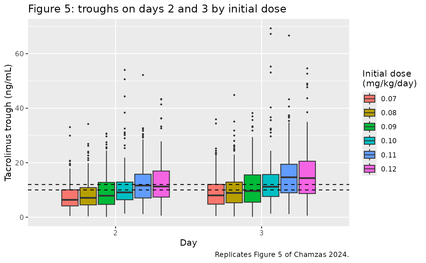
fig5_cmp <- troughs |>
  filter(day %in% c(2, 3), arm != "0.06") |>
  group_by(arm, day) |>
  summarise(sim_median = median(Cc), .groups = "drop") |>
  inner_join(fig5_published, by = c("arm", "day")) |>
  mutate(pct_diff = 100 * (sim_median - published_median) / published_median)

fig5_cmp |>
  select(day, arm, published_median, sim_median, pct_diff) |>
  arrange(day, arm) |>
  rename(
    "Day" = day, "Initial dose (mg/kg/day)" = arm,
    "Published median (ng/mL)" = published_median,
    "Simulated median (ng/mL)" = sim_median, "Difference (%)" = pct_diff
  ) |>
knitr::kable(digits = 1, caption = "Median trough: simulation vs. digitised Figure 5.")| Day | Initial dose (mg/kg/day) | Published median (ng/mL) | Simulated median (ng/mL) | Difference (%) |
|---|---|---|---|---|
| 2 | 0.07 | 6.5 | 6.4 | -2.0 |
| 2 | 0.08 | 7.4 | 7.1 | -4.1 |
| 2 | 0.09 | 8.2 | 7.9 | -3.8 |
| 2 | 0.10 | 9.2 | 9.1 | -1.0 |
| 2 | 0.11 | 10.2 | 11.6 | 13.9 |
| 2 | 0.12 | 10.8 | 11.3 | 4.3 |
| 3 | 0.07 | 7.8 | 8.0 | 2.7 |
| 3 | 0.08 | 9.3 | 8.9 | -4.2 |
| 3 | 0.09 | 10.5 | 9.6 | -8.7 |
| 3 | 0.10 | 11.6 | 11.2 | -3.7 |
| 3 | 0.11 | 12.5 | 14.7 | 17.2 |
| 3 | 0.12 | 13.6 | 14.4 | 5.5 |
stopifnot(
  # Structural: a mis-transcribed CL/F, volume or dose unit shifts every arm
  # by tens of percent. Typical-value troughs (every eta at zero) run 20-30%
  # above these medians, because the large BSV on Vc/F, Vp/F, Q/F and ktr
  # pulls the median trough below the typical-value trough.
  abs(median(fig5_cmp$pct_diff)) < 10,
  # Envelope across the twelve arm-days, robust to the cohort draw.
  quantile(abs(fig5_cmp$pct_diff), 0.9) < 25
)
The simulated spread for 0.10 mg/kg/day on day 3 is somewhat wider than the published box (about 8-15.5 ng/mL in Figure 5). The source reports that 27% of patients were inside 10-12 ng/mL and 18% were above 15 ng/mL on day 3 at this dose (Results 3.3.1). Those proportions come from the cohort’s own post-hoc parameters and covariates, so a virtual cohort is not expected to reproduce them exactly.
troughs |>
  filter(arm == "0.10", day == 3) |>
  summarise(
    p25 = quantile(Cc, 0.25), median = median(Cc), p75 = quantile(Cc, 0.75),
    pct_10_12 = 100 * mean(Cc >= 10 & Cc <= 12),
    pct_above_15 = 100 * mean(Cc > 15)
  ) |>
  rename(
    "P25 (ng/mL)" = p25, "Median (ng/mL)" = median, "P75 (ng/mL)" = p75,
    "% in 10-12 ng/mL" = pct_10_12, "% above 15 ng/mL" = pct_above_15
  ) |>
knitr::kable(digits = 1, caption = "Simulated day-3 troughs at 0.10 mg/kg/day.")| P25 (ng/mL) | Median (ng/mL) | P75 (ng/mL) | % in 10-12 ng/mL | % above 15 ng/mL |
|---|---|---|---|---|
| 7.6 | 11.2 | 15.7 | 17 | 29 |
Figure 3: trough at 72 h
The quantitative predictive check (Figure 3) compares the median observed trough in the 66-74 h window (about 8.3 ng/mL) with the median of 1,000 simulated datasets (about 8.7 ng/mL; median prediction error +5.01%). The patients in that window received their recorded doses: initial doses ranged from 0.02 to 0.14 mg/kg/day (median 0.06), and some had already been adjusted by 72 h. The closest virtual counterpart is the untitrated 0.06 mg/kg/day arm. It is shown for orientation only and is not used as a check, because its median runs 10-25% below 8.7 ng/mL across cohort draws. The dose history behind the published window is not available.
qpc <- troughs |>
  filter(arm == "0.06", time == 72) |>
  summarise(median_trough = median(Cc))
knitr::kable(
  rename(qpc, "Simulated median trough at 72 h (ng/mL)" = median_trough),
  digits = 2,
  caption = "Median 72-h trough, untitrated 0.06 mg/kg/day; published observed median 8.3 ng/mL, simulated 8.7 ng/mL."
)| Simulated median trough at 72 h (ng/mL) |
|---|
| 6.82 |
Figures 6-8: titration strategies
Figures 6 and 7 apply the recommended titration protocol in Table 3. Figure 8 applies the hospital’s current titration protocol, which the source does not publish. Neither is reproduced here, because both depend on per-patient post-hoc parameters and on scheduling rules that the source does not fully specify, such as when a measured trough triggers an adjustment, and on which day the adjusted dose is next re-measured.
PKNCA validation
The source reports no NCA. This check confirms internal consistency
at steady state. Over one 12-h dosing interval, AUC0-12 must equal Dose
/ (CL/F) for each subject. Doses are given at steady state
(ss = 1) and sampled on a dense grid.
nca_events <- bind_rows(lapply(c(0.06, 0.10), function(d) {
  covs |>
    slice_head(n = 100) |>
    mutate(
      id = seq_len(n()) + if (d == 0.06) 0L else 100L,
      treatment = sprintf("%.2f mg/kg/day", d),
      amt = pmax(0.5, round(WT * d / 2 / 0.5) * 0.5)
    )
})) |>
  (\(subj) bind_rows(
    subj |> mutate(time = 0, evid = 1L, ss = 1L, ii = 12, cmt = "depot"),
    subj |>
      tidyr::expand_grid(obs_time = seq(0, 12, by = 0.1)) |>
      mutate(time = obs_time, evid = 0L, amt = 0, ss = 0L, ii = 0, cmt = "central") |>
      select(-obs_time)
  ))() |>
  arrange(id, time, desc(evid))

# steady-state searches for long-half-life subjects exceed the default step budget
sim_ss <- rxode2::rxSolve(mod, events = nca_events, keep = c("treatment"), maxsteps = 1e6) |>
  as.data.frame()

# A subject that fails to solve comes back NA; stop rather than drop it.
stopifnot(!anyNA(sim_ss$Cc))
conc_df <- sim_ss |>
  filter(!is.na(Cc)) |>
  select(id, time, Cc, treatment)
dose_df <- nca_events |>
  filter(evid == 1) |>
  select(id, time, amt, treatment)

conc_obj <- PKNCA::PKNCAconc(conc_df, Cc ~ time | treatment + id)
dose_obj <- PKNCA::PKNCAdose(dose_df, amt ~ time | treatment + id)
intervals <- data.frame(
  start = 0, end = 12,
  cmax = TRUE, tmax = TRUE, cmin = TRUE, auclast = TRUE
)
nca_res <- PKNCA::pk.nca(PKNCA::PKNCAdata(conc_obj, dose_obj, intervals = intervals))

nca_wide <- as.data.frame(nca_res) |>
  select(treatment, id, PPTESTCD, PPORRES) |>
  tidyr::pivot_wider(names_from = PPTESTCD, values_from = PPORRES)

nca_wide |>
  group_by(treatment) |>
  summarise(
    cmax = median(cmax), tmax = median(tmax), cmin = median(cmin),
    auclast = median(auclast), .groups = "drop"
  ) |>
  rename(
    "Regimen" = treatment, "Cmax (ng/mL)" = cmax, "Tmax (h)" = tmax,
    "Cmin (ng/mL)" = cmin, "AUC0-12 (ng*h/mL)" = auclast
  ) |>
knitr::kable(digits = 2, caption = "Steady-state NCA (medians across subjects).")| Regimen | Cmax (ng/mL) | Tmax (h) | Cmin (ng/mL) | AUC0-12 (ng*h/mL) |
|---|---|---|---|---|
| 0.06 mg/kg/day | 18.01 | 1.35 | 8.57 | 129.65 |
| 0.10 mg/kg/day | 32.12 | 1.10 | 16.90 | 246.95 |
# AUC0-12 at steady state = Dose / (CL/F); mg / (L/h) * 1000 = ng*h/mL.
auc_chk <- sim_ss |>
  distinct(id, cl) |>
  inner_join(distinct(dose_df, id, amt), by = "id") |>
  inner_join(nca_wide, by = "id") |>
  mutate(pct_err = 100 * (auclast - amt * 1000 / cl) / (amt * 1000 / cl))
stopifnot(
  # Same drawn parameters on both sides: only trapezoid error on a 0.1 h grid
  # (observed 90th percentile about 0.005% across cohort draws).
  abs(median(auc_chk$pct_err)) < 0.1,
  quantile(abs(auc_chk$pct_err), 0.9) < 0.5
)
summary(auc_chk$pct_err)
#>       Min.    1st Qu.     Median       Mean    3rd Qu.       Max.
#> -0.1484071 -0.0013412 -0.0005984 -0.0024600 -0.0002648  0.0106449
Assumptions and deviations
- Transit chain. The source states that “three transit compartments” fit the rich data and reports only one rate constant (Ktr), with no separate absorption rate. The package follows the reading used for the Benkali 2010 and Woillard 2011 tacrolimus models (both cited by the source as the same structure): the dose enters the first of three compartments, and each compartment, including the last, transfers at ktr. An alternative reading, with three transit compartments after a separate dosing depot (four transfers at ktr), changes the simulated typical troughs at 0.1 mg/kg/day by less than 1% and the steady-state Cmax by less than 0.5%. The maintainers checked both readings, and the difference is immaterial for this trough-based model.
-
BSV scale. Table 2 reports %BSV without a
definition. The variances are taken as
log(1 + (%BSV/100)^2). This gives the round values 0.470, 0.880, 0.714, 0.755 and 0.558, which suggests the authors reported the exponential-scale CV of round omega^2 values. Reading %BSV as sqrt(omega^2) instead would give variances of 0.60 to 1.41. - Vp/F and Q/F precision. Results 3.1 gives Vp/F = 325.6 L and Q/F = 62.5 L/h, while Table 2 gives 325 L and 62.46 L/h. The more precise value of each is used.
- Hematocrit reference. Equation 5 centres hematocrit on “HCT_median” without printing the number. The Abstract and Supplementary Table S2 name the typical patient as having 30% hematocrit, and Table 1 reports a cohort mean of 30.0%. The model uses 30%, which reproduces all four Supplementary Table S2 fold-changes.
- Hematocrit is time-varying in the source. The virtual cohort holds each patient’s hematocrit constant. Supply HCT per record (in percent) to simulate its post-transplant recovery.
- Bioavailability. All disposition parameters are apparent (divided by F), and no bioavailability term is carried.
- Residual error. Table 2 reports an additive residual error only (2.62 ng/mL). The simulations above use individual predictions without residual error, as the source did for its dose-finding simulations.
- Virtual cohort. Weight and hematocrit are drawn from normal distributions with the Table 1 means and SDs, truncated to 40-160 kg and 15-50%, and drawn independently of each other.
- Not reproduced. The titration-protocol simulations (Figures 6-8) are described above. The source reports no NCA, so the PKNCA section checks internal steady-state consistency instead of comparing against published values.
- Europe PMC lists no erratum or correction notice for this article as of 2026-10-30.