SPT-07A (D-borneol) whole-body PBPK in rats, dogs and humans (Zhu 2024)
Source:vignettes/articles/Zhu_2024_borneol_pbpk.Rmd
Zhu_2024_borneol_pbpk.RmdModel and source
Zhu 2024 builds a single whole-body PBPK structure and parameterises it three times – once per species – so the paper contributes three model files that share this vignette.
model_names <- c(
  rat   = "Zhu_2024_borneol_rat_pbpk",
  dog   = "Zhu_2024_borneol_dog_pbpk",
  human = "Zhu_2024_borneol_human_pbpk"
)
# readModelDb() returns the model FUNCTION; rxode2::rxode() resolves it to a ui.
uis <- lapply(model_names, function(nm) rxode2::rxode(readModelDb(nm)))- Citation: Zhu X, Kong W, Wang Z, Liu X, Liu L. (2024). Prediction of SPT-07A Pharmacokinetics in Rats, Dogs, and Humans Using a Physiologically-Based Pharmacokinetic Model and In Vitro Data. Pharmaceutics 16(12):1596. doi:10.3390/pharmaceutics16121596. PMCID PMC11676658. Model equations: Equations (7)-(16), pages 7-8. Rat physiology (volumes, blood flows, tissue:plasma partition coefficients, Rb, fu,p): Table 1, ‘Rat (0.25 kg)’ columns. Unbound whole-organ intrinsic clearances: Table 2, rat rows (RLMs / RKMs / RIMs). The adipose permeability-surface product PS is NOT reported anywhere in the paper; it is recovered by digitising the paper’s own rat adipose simulation (Figure 4J) – see the inline note on PS and the vignette Errata. No erratum or corrigendum was located for this article.
- Article: https://doi.org/10.3390/pharmaceutics16121596
- PMC full text: https://www.ncbi.nlm.nih.gov/pmc/articles/PMC11676658/
There is no supplementary material for this article, and no erratum or corrigendum was located.
SPT-07A is D-borneol, a bicyclic monoterpene in development in China for acute ischaemic stroke. The model is built bottom-up from in vitro metabolism data: SPT-07A is cleared almost entirely by UDP-glucuronosyltransferase (UGT) glucuronidation, and unusually the kidney and intestine carry a substantial share of it, which is what motivated the whole-body treatment. All tissues are perfusion-rate limited except adipose, which is permeability-limited because rat tissue-distribution work showed marked adipose accumulation.
rat – Preclinical (rat, Sprague-Dawley). PBPK
(whole-body, Phoenix WinNonlin 8.3). SPT-07A (D-borneol), a bicyclic
monoterpene under development in China for acute ischaemic stroke, after
intravenous bolus dosing. Fourteen mass-balance compartments (lung,
heart, brain, muscle, skin, adipose, kidney, spleen, stomach, liver,
intestine, rest of body, plus arterial and venous blood) built entirely
from in vitro and in silico data: every tissue except adipose is
perfusion-rate limited, and adipose is permeability-limited (a vascular
sub-compartment vp_adipose exchanging with the
extravascular tissue adipose through a permeability-surface
product PS), because rat tissue-distribution studies showed high adipose
accumulation. Elimination occurs in three organs – liver, kidney and
intestine – as unbound whole-organ intrinsic clearances measured in rat
liver, kidney and intestinal microsomes and scaled by MPPGL / MPPGK /
MPPGI; SPT-07A is cleared almost entirely by UDP-glucuronosyltransferase
glucuronidation (hepatic UGT CLint,u 2060 vs CYP 5.14 uL/min/mg
protein), with the liver, kidney and intestine contributing 62.2%, 32.6%
and 5.2% of systemic clearance. Tissue:plasma partition coefficients
were computed by the Schmitt tissue-composition method, not fitted. This
is the species the model was BUILT and validated on before being scaled
to dog and human (see modellib(‘Zhu_2024_borneol_dog_pbpk’) and
modellib(‘Zhu_2024_borneol_human_pbpk’)); PS is the single parameter
estimated from in vivo data (fitted to rat adipose concentrations) and
the two other species inherit it by body-weight scaling. Deterministic
typical-value simulator: the paper’s 5th-95th percentile bands come from
100 virtual subjects whose variability magnitude is never reported, so
no IIV and no residual error are encoded (see the vignette Errata).
dog – Preclinical (beagle dog). PBPK (whole-body, Phoenix WinNonlin 8.3). SPT-07A (D-borneol), a bicyclic monoterpene under development in China for acute ischaemic stroke, after intravenous bolus dosing. Structurally IDENTICAL to the rat model that was built first (see modellib(‘Zhu_2024_borneol_rat_pbpk’)): fourteen mass-balance compartments, perfusion-rate-limited distribution everywhere except a permeability-limited adipose, and elimination in liver, kidney and intestine as unbound whole-organ intrinsic clearances. What changes is (a) beagle physiology (Table 1 dog column) and (b) dog-specific in vitro intrinsic clearances (Table 2 DLMs / DKMs). This is a pure FORWARD SCALE-UP, not a refit: nothing was estimated from dog in vivo data, and the one in-vivo-fitted parameter in the whole model – the adipose permeability-surface product PS – is inherited from the rat by linear body-weight scaling (Equation 13), which is what makes the dog plasma predictions a genuine cross-species test. NO intestinal elimination: glucuronidation of SPT-07A was not detectable in dog intestinal microsomes (Table 2 DIMs row is ‘-’), so CLintIntestine is fixed at zero and the dog clears the drug through liver (87.3%) and kidney (12.7%) only. Dog hepatic glucuronidation is by far the fastest of the three species (UGT CLint,u 12,200 uL/min/mg protein vs 2060 in rat and 745 in human). Deterministic typical-value simulator: no IIV and no residual error are encoded (see the vignette Errata).
human – PBPK (whole-body, Phoenix WinNonlin 8.3). SPT-07A (D-borneol), a bicyclic monoterpene under development in China for acute ischaemic stroke, in healthy adults after intravenous infusion. Structurally IDENTICAL to the rat model the framework was built on (see modellib(‘Zhu_2024_borneol_rat_pbpk’)): fourteen mass-balance compartments, perfusion-rate-limited distribution everywhere except a permeability-limited adipose, and elimination in liver, kidney and intestine as unbound whole-organ intrinsic clearances. What changes is (a) human physiology (Table 1 human column) and (b) human-specific in vitro intrinsic clearances (Table 2 HLMs / HKMs / HIMs). This is a pure BOTTOM-UP PREDICTION: no human in vivo data were used to build or fit it – the clinical data it is compared against are cited from a separate first-in-human study – and the one in-vivo-fitted parameter, the adipose permeability-surface product PS, is inherited from the rat by linear body-weight scaling (Equation 13). SPT-07A is cleared predominantly by UGT glucuronidation (hepatic UGT CLint,u 745 vs CYP 3.35 uL/min/mg protein), with liver, kidney and intestine contributing 76.5%, 23.1% and 0.4% of systemic clearance; UGT phenotyping identified UGT1A1 and UGT2B7 as the responsible isoforms, though a relative-activity-factor reconstruction recovers only ~36% of the measured hepatic activity, implying additional uncharacterised UGTs. The notably high renal contribution is consistent with the paper’s opening observation that the reported human clearance (1942 mL/min) exceeds hepatic blood flow (1450 mL/min). Deterministic typical-value simulator: no IIV and no residual error are encoded (see the vignette Errata).
Population
The three species were studied as follows (Methods 2.3.1-2.3.4). Rats (258 Sprague-Dawley animals across the kinetic and tissue-distribution studies) received 0.5, 1 and 2 mg/kg as a single IV bolus plus a 1 mg/kg qd multiple-dose arm, with plasma sampled to 240 min. Six beagle dogs received 0.25, 0.5 and 1 mg/kg as single IV boluses in a three-period cross-over, plus a multiple-dose arm, with plasma sampled to 300 min. The human data are not original to this paper – Methods 2.3.4 states they were cited from the paper’s reference [7]: 36 healthy volunteers in three cohorts of 12 received 10, 20 or 40 mg as a 1 h IV infusion, single dose on day 0 and then q12h for 7 days beginning at 48 h.
Two sampling details matter for the validation below: rats and dogs received an IV bolus with the first sample at 5 min, whereas humans received a 1 h infusion. That difference is the whole explanation for the Table 3 discrepancy discussed in the Errata.
str(uis$human$population)
#> List of 11
#>  $ species       : chr "human"
#>  $ n_subjects    : int 36
#>  $ n_studies     : int 1
#>  $ age_range     : chr NA
#>  $ weight_range  : chr "70 kg reference adult (Table 1)"
#>  $ sex_female_pct: num NA
#>  $ race_ethnicity: chr "Not reported (study conducted in China)"
#>  $ disease_state : chr "Healthy volunteers"
#>  $ dose_range    : chr "10, 20 and 40 mg as a 1 h IV infusion; single dose on day 0, then q12h for 7 days from 48 h"
#>  $ regions       : chr "China"
#>  $ notes         : chr "Methods 2.3.4: the clinical data are NOT original to this paper -- they are cited from the paper's reference [7"| __truncated__
Source trace
Every ini() entry carries an in-file comment naming its
source location; the table below collects the model-level provenance in
one place.
| Equation / parameter block | Source location |
|---|---|
| Perfusion-limited tissue ODE | Equation (7), page 7 |
| Arterial blood ODE | Equation (8), page 7 |
| Venous blood ODE | Equation (9), page 7 |
| Lung ODE | Equation (10), page 7 |
Adipose vascular sub-compartment ODE (vp_adipose,
paper’s C1) |
Equation (11), page 7 |
Adipose extravascular ODE (adipose, paper’s C2) |
Equation (12), page 7 |
Interspecies PS scaling
PS_i = PS_rat * (W_i / W_rat)
|
Equation (13), page 7 |
| Liver ODE (eliminating, receives splanchnic inflow) | Equation (14), page 7 |
| Kidney ODE (eliminating) | Equation (15), page 8 |
| Intestine ODE (eliminating) | Equation (16), page 8 |
Organ volumes, blood flows, Kt:pl, Rb,
fu,p (all 3 species) |
Table 1 |
Adipose V1 / V2 split (all 3 species) |
Paper text below Equation (12) (PK-Sim 11.2) |
| Unbound whole-organ intrinsic clearances (all 3 species) | Table 2, CL int, in vivo,u column |
| Well-stirred organ clearances used as a check below | Results 3.1.3 |
| Predicted vs observed Cmax / AUC / CL / t1/2 | Table 3 |
PS (adipose permeability-surface product) |
Not reported anywhere – back-solved from Figure 4J; see Errata |
Structural checks
Before comparing against published exposures, two checks confirm the physiology and the elimination algebra were transcribed correctly. Both are exact arithmetic identities, so they either hold or they do not.
Blood-flow mass balance
Every tissue flow must sum to the cardiac output printed on the Table 1 lung row, and the printed total hepatic inflow must equal the hepatic artery plus the three splanchnic organs that drain into the liver.
flow_check <- lapply(names(uis), function(sp) {
  th <- uis[[sp]]$theta
  tissue_sum <- sum(th[c("Qheart", "Qbrain", "Qmuscle", "Qadipose", "Qskin",
                         "Qkidney", "Qother", "Qhepart", "Qspleen", "Qstomach",
                         "Qintestine")])
  liver_in <- sum(th[c("Qhepart", "Qspleen", "Qstomach", "Qintestine")])
  data.frame(
    Species             = sp,
    `Sum of tissue flows` = tissue_sum,
    `Cardiac output (Table 1)` = unname(th["Qtotal"]),
    `Difference (%)`    = 100 * (tissue_sum - th["Qtotal"]) / th["Qtotal"],
    `Total hepatic inflow` = liver_in,
    check.names = FALSE
  )
}) |> dplyr::bind_rows()

knitr::kable(
  flow_check, digits = 3, row.names = FALSE,
  caption = paste(
    "Blood-flow mass balance. The rat closes exactly; the dog and human tables",
    "carry small rounding differences (0.13% and 0.006%) which are reproduced",
    "as printed rather than silently reconciled. Total hepatic inflow matches",
    "the Table 1 'Liver' blood-flow row exactly in all three species",
    "(rat 12.30, dog 323.33, human 1518.33 mL/min)."
  )
)| Species | Sum of tissue flows | Cardiac output (Table 1) | Difference (%) | Total hepatic inflow |
|---|---|---|---|---|
| rat | 83.90 | 83.9 | 0.000 | 12.30 |
| dog | 1121.46 | 1120.0 | 0.130 | 323.33 |
| human | 5600.33 | 5600.0 | 0.006 | 1518.33 |
Well-stirred organ clearances
Equations (14)-(16) drive elimination with the plasma-equivalent
concentration C_t / K_t:pl, so each eliminating organ
behaves as a well-stirred compartment with blood clearance
Q * fu,b * CLint / (Q + fu,b * CLint), where
fu,b = fu,p / Rb. Reproducing the paper’s own Results 3.1.3
numbers from the packaged ini() values is a direct test
that the elimination term was encoded correctly.
well_stirred <- function(ui, organ) {
  th <- ui$theta
  clint <- unname(th[paste0("CLint", organ)]) * unname(th["BW"])
  fub   <- unname(th["fup"]) / unname(th["Rb"])
  q <- switch(organ,
    Liver     = sum(th[c("Qhepart", "Qspleen", "Qstomach", "Qintestine")]),
    Kidney    = unname(th["Qkidney"]),
    Intestine = unname(th["Qintestine"])
  )
  unname(q * fub * clint / (q + fub * clint) / th["BW"])
}

# Results 3.1.3, mL/min/kg. Dog intestine is absent (no glucuronidation in DIMs).
published_cl <- tibble::tribble(
  ~Species, ~Organ,      ~Published,
  "rat",    "Liver",     46.6,
  "rat",    "Kidney",    24.4,
  "rat",    "Intestine", 3.90,
  "dog",    "Liver",     37.8,
  "dog",    "Kidney",    5.50,
  "human",  "Liver",     20.4,
  "human",  "Kidney",    6.14,
  "human",  "Intestine", 0.109
)

cl_check <- published_cl |>
  dplyr::mutate(
    Recomputed = mapply(function(s, o) well_stirred(uis[[s]], o), Species, Organ),
    `% diff`   = 100 * (Recomputed - Published) / Published
  )

knitr::kable(
  cl_check, digits = c(0, 0, 3, 3, 2),
  caption = paste(
    "Well-stirred organ blood clearances (mL/min/kg) recomputed from the",
    "packaged ini() values versus the values the paper reports in Results",
    "3.1.3. All eight agree to the printed precision."
  )
)| Species | Organ | Published | Recomputed | % diff |
|---|---|---|---|---|
| rat | Liver | 46.600 | 46.607 | 0.02 |
| rat | Kidney | 24.400 | 24.447 | 0.19 |
| rat | Intestine | 3.900 | 3.905 | 0.13 |
| dog | Liver | 37.800 | 37.837 | 0.10 |
| dog | Kidney | 5.500 | 5.502 | 0.05 |
| human | Liver | 20.400 | 20.363 | -0.18 |
| human | Kidney | 6.140 | 6.142 | 0.03 |
| human | Intestine | 0.109 | 0.109 | -0.12 |
Simulation
The models are deterministic typical-value simulators: the paper
never reports the magnitude of the parameter variability behind its
5th-95th percentile bands, so no IIV and no residual error are encoded.
Every simulation below is therefore a single typical subject per dose
arm (omega = NA is not passed – these models
declare no etas).
solve_arm <- function(ui, dose_mg, times, infusion_min = 0, dose_times = 0) {
  rate_val <- if (infusion_min > 0) dose_mg / infusion_min else 0
  dosing <- data.frame(
    time = dose_times, amt = dose_mg, evid = 1L,
    cmt = "venous", rate = rate_val
  )
  obs <- data.frame(
    time = times, amt = NA_real_, evid = 0L,
    cmt = "venous", rate = 0            # ODE state name, never the observable "Cc"
  )
  ev <- dplyr::arrange(dplyr::bind_rows(dosing, obs), time, dplyr::desc(evid))
  rxode2::rxSolve(ui, ev, atol = 1e-10, rtol = 1e-10, returnType = "data.frame")
}

# A grid that resolves the post-bolus distribution phase finely enough for NCA.
grid_for <- function(tmax) {
  g <- c(
    seq(0, 5, by = 0.05), seq(5, 60, by = 0.25),
    seq(60, 600, by = 2), seq(600, max(tmax, 600), by = 10)
  )
  sort(unique(g[g <= tmax]))
}
arms <- tibble::tribble(
  ~species, ~dose_label,  ~dose_mg,        ~infusion_min,
  "rat",    "0.5 mg/kg",  0.5   * 0.25,    0,
  "rat",    "1 mg/kg",    1     * 0.25,    0,
  "rat",    "2 mg/kg",    2     * 0.25,    0,
  "dog",    "0.25 mg/kg", 0.25  * 8.5,     0,
  "dog",    "0.5 mg/kg",  0.5   * 8.5,     0,
  "dog",    "1 mg/kg",    1     * 8.5,     0,
  "human",  "10 mg",      10,              60,
  "human",  "20 mg",      20,              60,
  "human",  "40 mg",      40,              60
)

TMAX <- 6000  # min; >= 15 terminal half-lives in every species
sims <- arms |>
  dplyr::rowwise() |>
  dplyr::group_map(function(a, ...) {
    solve_arm(uis[[a$species]], a$dose_mg, grid_for(TMAX), a$infusion_min) |>
      dplyr::mutate(species = a$species, dose_label = a$dose_label,
                    dose_mg = a$dose_mg)
  }) |>
  dplyr::bind_rows() |>
  dplyr::mutate(arm = paste(species, dose_label))
Plasma concentration-time profiles (Figures 3, 5 and 6)
sims |>
  dplyr::filter(!dplyr::near(time, 0), time <= 300, Cc > 1e-12) |>
  dplyr::mutate(species = factor(species, c("rat", "dog", "human"))) |>
  ggplot(aes(time, Cc * 1000, colour = dose_label)) +
  geom_line(linewidth = 0.7) +
  facet_wrap(~species, scales = "free_y") +
  scale_y_log10() +
  labs(x = "Time (min)", y = "Plasma SPT-07A (ng/mL)", colour = "Dose") +
  theme_bw() +
  theme(legend.position = "bottom")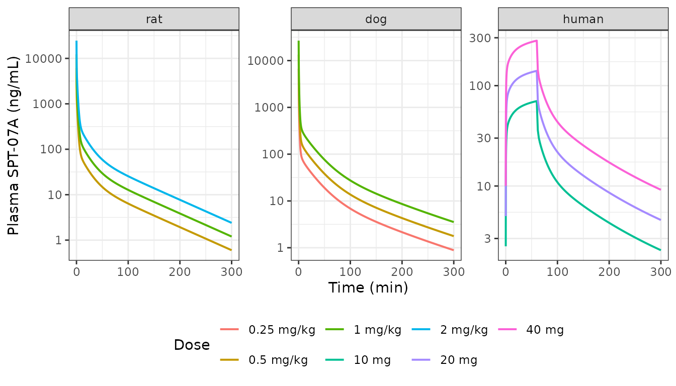
Replicates Figure 3 (rats), Figure 5 (dogs) and Figure 6 (humans) of Zhu 2024: simulated typical-value plasma SPT-07A after single intravenous doses.
Rat tissue distribution (Figure 4)
Figure 4 of the paper shows plasma plus ten tissues in rats after 2
mg/kg. The adipose panel (4J) is the one that carries information about
PS: it is the only tissue whose simulated profile
rises to a peak rather than declining monotonically, which is
the signature of permeability-limited uptake.
rat2 <- solve_arm(uis$rat, 2 * 0.25, grid_for(300))
th_rat <- uis$rat$theta

tissue_conc <- rat2 |>
  dplyr::transmute(
    time,
    plasma    = Cc,
    heart     = heart     / (th_rat[["Vheart"]]     * 1e-3),
    liver     = liver     / (th_rat[["Vliver"]]     * 1e-3),
    spleen    = spleen    / (th_rat[["Vspleen"]]    * 1e-3),
    stomach   = stomach   / (th_rat[["Vstomach"]]   * 1e-3),
    brain     = brain     / (th_rat[["Vbrain"]]     * 1e-3),
    intestine = intestine / (th_rat[["Vintestine"]] * 1e-3),
    muscle    = muscle    / (th_rat[["Vmuscle"]]    * 1e-3),
    lung      = lung      / (th_rat[["Vlung"]]      * 1e-3),
    adipose   = adipose   / (th_rat[["Vadipose2"]]  * 1e-3),
    kidney    = kidney    / (th_rat[["Vkidney"]]    * 1e-3)
  ) |>
  tidyr::pivot_longer(-time, names_to = "tissue", values_to = "conc") |>
  dplyr::filter(!dplyr::near(time, 0), conc > 1e-12)

ggplot(tissue_conc, aes(time, conc * 1000)) +
  geom_line(linewidth = 0.6) +
  facet_wrap(~tissue, scales = "free_y", ncol = 4) +
  scale_y_log10() +
  labs(x = "Time (min)", y = "Concentration (ng/mL or ng/g)") +
  theme_bw()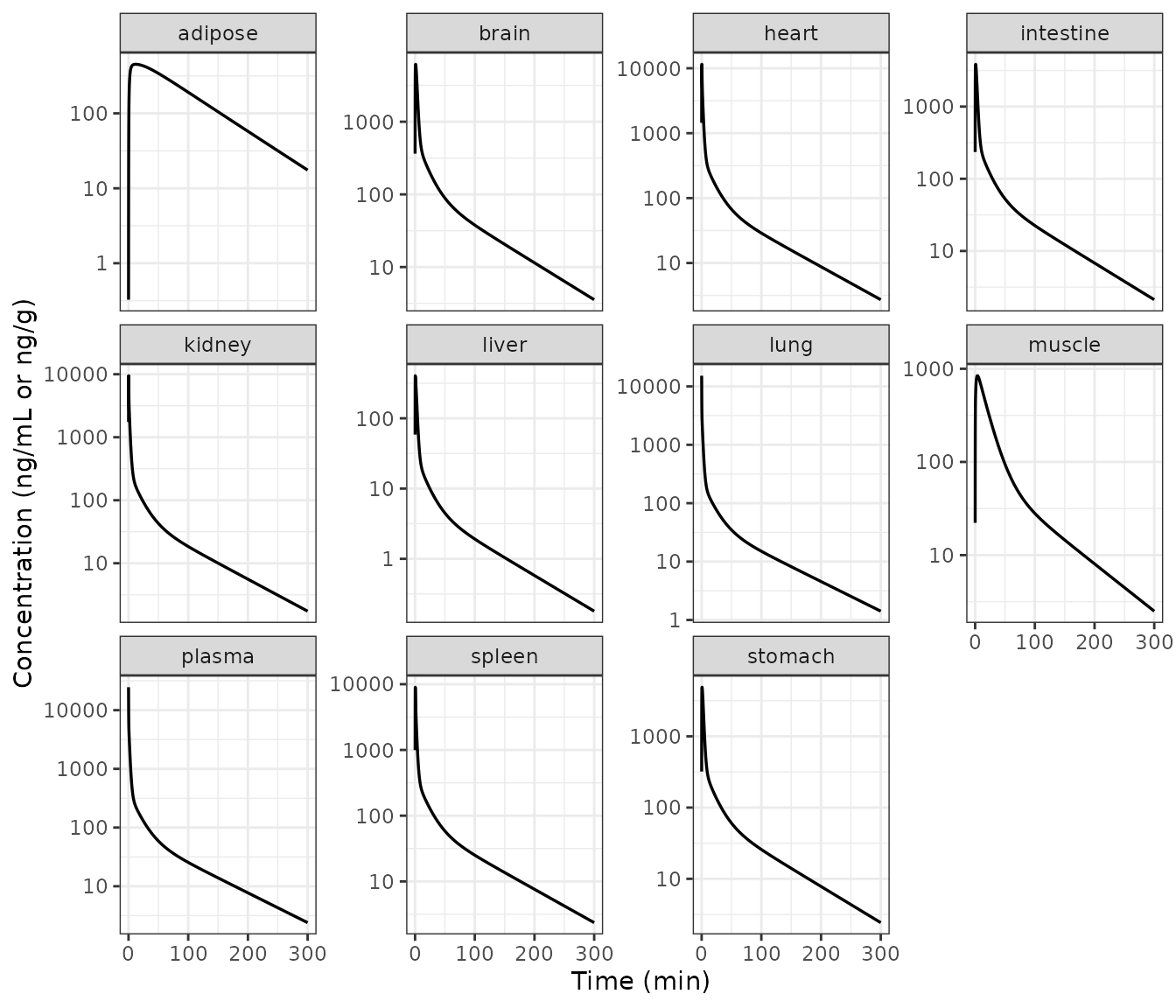
Replicates Figure 4B-K of Zhu 2024: simulated typical-value tissue concentrations in the rat after a 2 mg/kg IV bolus.
Recovering PS from Figure 4J
PS is the single parameter in the whole model that was
fitted to in vivo data, and its value is not reported. It was recovered
by digitising the median line of Figure 4J and solving for the
PS that reproduces it; the optimiser returns 0.499 mL/min,
i.e. the authors’ round 0.5. The digitised points are reproduced below
with their provenance so a reviewer can audit the back-solve.
# Digitised from Figure 4J (rat adipose, 2 mg/kg IV bolus), median line.
fig4j <- tibble::tibble(
  time = c(5, 30, 60, 90),
  conc = c(430, 410, 278, 205)     # ng/g
)

adipose_pred <- tissue_conc |>
  dplyr::filter(tissue == "adipose") |>
  dplyr::mutate(conc_ng = conc * 1000)

ps_cmp <- fig4j |>
  dplyr::mutate(
    Simulated = approx(adipose_pred$time, adipose_pred$conc_ng, xout = time)$y,
    `% diff`  = 100 * (Simulated - conc) / conc
  ) |>
  dplyr::rename("Time (min)" = time, "Digitised Fig 4J (ng/g)" = conc)

knitr::kable(ps_cmp, digits = c(0, 0, 1, 1),
caption = "Back-solved PS = 0.5 mL/min against the digitised Figure 4J median.")| Time (min) | Digitised Fig 4J (ng/g) | Simulated | % diff |
|---|---|---|---|
| 5 | 430 | 421.3 | -2.0 |
| 30 | 410 | 413.7 | 0.9 |
| 60 | 278 | 305.8 | 10.0 |
| 90 | 205 | 215.4 | 5.1 |
ggplot(adipose_pred, aes(time, conc_ng)) +
  geom_line(linewidth = 0.7) +
  geom_point(data = fig4j, aes(time, conc), colour = "firebrick", size = 2.5) +
  labs(x = "Time (min)", y = "Rat adipose SPT-07A (ng/g)",
       subtitle = "Line: packaged model. Points: digitised Figure 4J median.") +
  theme_bw()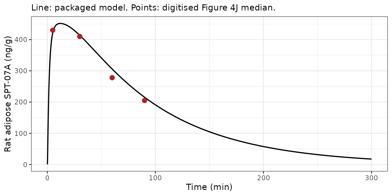
Simulated rat adipose (extravascular) concentration at the back-solved PS = 0.5 mL/min versus the digitised median line of Figure 4J.
PKNCA validation against Table 3
nca_input <- sims |>
  dplyr::filter(!is.na(Cc)) |>
  dplyr::mutate(id = arm) |>
  # Per arm, keep Cc >= 1e-6 * Cmax after the peak: below that the ODE integrator has no relative accuracy left.
  dplyr::group_by(id) |>
  dplyr::filter(time <= time[which.max(Cc)] | Cc >= 1e-6 * max(Cc)) |>
  dplyr::ungroup()

dose_input <- arms |>
  dplyr::mutate(id = paste(species, dose_label), time = 0) |>
  dplyr::select(id, time, dose_mg, species, dose_label)

conc_obj <- PKNCA::PKNCAconc(nca_input, Cc ~ time | id)
dose_obj <- PKNCA::PKNCAdose(as.data.frame(dose_input), dose_mg ~ time | id)

intervals <- data.frame(
  start = 0, end = Inf,
  cmax = TRUE, aucinf.obs = TRUE
)

res <- PKNCA::pk.nca(PKNCA::PKNCAdata(conc_obj, dose_obj, intervals = intervals))

# PKNCA also returns the DEPENDENCIES of the requested parameters -- notably its
# own `half.life` / `lambda.z`, which aucinf.obs needs. Those extra rows must be
# dropped: a windowed half-life is appended below, and leaving PKNCA's
# asymptotic one in place would silently produce two half.life rows per arm,
# which ncaComparisonTable() would then average.
nca <- as.data.frame(res) |>
  dplyr::filter(PPTESTCD %in% c("cmax", "aucinf.obs")) |>
  dplyr::select(id, PPTESTCD, PPORRES) |>
  dplyr::left_join(dose_input, by = "id")
Terminal half-life is deliberately not taken from a 0-Inf PKNCA interval. This model has a slowly-equilibrating adipose compartment, so its true asymptotic terminal slope (rat 60, dog 139, human 217 min) is much shallower than anything a finite study could observe; comparing that against a published half-life would compare two different quantities.
Instead one uniform rule is applied to all three species – fit the terminal slope over the final half of that species’ sampling window – and the resulting windows are stated explicitly. Rats were sampled to 240 min and dogs to 300 min (Methods 2.3.1 and 2.3.3). The clinical sampling schedule is not given in this paper (the human data are cited from reference [7]), so a 12 h window is assumed, consistent with the q12h multiple-dose regimen. The rule is fixed in advance and applied identically to every species rather than tuned per arm.
# end of the sampling window (min); the slope is fitted over the final half
hl_end   <- c(rat = 240, dog = 300, human = 720)
hl_start <- hl_end / 2

half_life_windowed <- sims |>
  dplyr::group_by(species, dose_label) |>
  dplyr::group_modify(function(d, k) {
    sp <- k$species
    # Keep Cc >= 1e-6 * Cmax: below that the ODE integrator has no relative accuracy left.
    w <- d[d$time >= hl_start[[sp]] & d$time <= hl_end[[sp]] & d$Cc >= 1e-6 * max(d$Cc, na.rm = TRUE), ]
    data.frame(PPTESTCD = "half.life",
               PPORRES  = unname(log(2) / -coef(lm(log(w$Cc) ~ w$time))[2]))
  }) |>
  dplyr::ungroup()

nca <- dplyr::bind_rows(nca, half_life_windowed)

# Guard against the duplicate-row trap above: ncaComparisonTable() takes the
# MEDIAN over repeated (group, parameter) rows, so a stray duplicate would be
# silently averaged rather than reported or flagged.
stopifnot(!any(duplicated(nca[, c("species", "dose_label", "PPTESTCD")])))
Table 3 reports predicted Cmax (humans only – the animal arms were IV boluses, for which the paper tabulates no Cmax), AUC and terminal half-life. The comparison below uses the paper’s predicted column, since reproducing the authors’ own simulation is what validates the packaged implementation.
# Zhu 2024 Table 3, "Pre" (predicted) columns.
# AUC in ug*min/mL == mg*min/L, which is the unit of Cc * time here.
published <- tibble::tribble(
  ~species, ~dose_label,  ~cmax,     ~aucinf.obs, ~half.life,
  "rat",    "0.5 mg/kg",  NA_real_,  3.78,        NA_real_,
  "rat",    "1 mg/kg",    NA_real_,  7.56,        58.2,
  "rat",    "2 mg/kg",    NA_real_,  15.1,        58.2,
  "dog",    "0.25 mg/kg", NA_real_,  3.60,        NA_real_,
  "dog",    "0.5 mg/kg",  NA_real_,  7.19,        76.7,
  "dog",    "1 mg/kg",    NA_real_,  14.4,        NA_real_,
  "human",  "10 mg",      0.0701,    5.76,        179,
  "human",  "20 mg",      0.1400,    11.5,        179,
  "human",  "40 mg",      0.2810,    23.0,        179
) |>
  tidyr::pivot_longer(c(cmax, aucinf.obs, half.life),
                      names_to = "PPTESTCD", values_to = "PPORRES") |>
  dplyr::filter(!is.na(PPORRES))

cmp <- nlmixr2lib::ncaComparisonTable(
  simulated     = dplyr::select(nca, species, dose_label, PPTESTCD, PPORRES),
  reference     = published,
  by            = c("species", "dose_label"),
  units         = c(cmax = "mg/L", aucinf.obs = "mg*min/L", half.life = "min"),
  tolerance_pct = 20
)

cmp |>
  dplyr::rename("Species" = species, "Dose" = dose_label) |>
  knitr::kable(
    caption = paste(
      "Simulated NCA from the packaged models versus the PREDICTED column of",
      "Zhu 2024 Table 3. * marks a difference above 20%. The human arms -- the",
      "only ones dosed as an infusion -- agree throughout; every starred row is",
      "a rat or dog AUC, for the reason set out in the Errata."
    ),
    align = c("l", "l", "l", "r", "r", "r")
)| NCA parameter | Species | Dose | Reference | Simulated | % diff |
|---|---|---|---|---|---|
| Cmax (mg/L) | human | 10 mg | 0.0701 | 0.0702 | +0.1% |
| Cmax (mg/L) | human | 20 mg | 0.14 | 0.14 | +0.3% |
| Cmax (mg/L) | human | 40 mg | 0.281 | 0.281 | -0.1% |
| AUC0-∞ (obs) (mg*min/L) | rat | 0.5 mg/kg | 3.78 | 6.38 | +68.8%* |
| AUC0-∞ (obs) (mg*min/L) | rat | 1 mg/kg | 7.56 | 12.8 | +68.8%* |
| AUC0-∞ (obs) (mg*min/L) | rat | 2 mg/kg | 15.1 | 25.5 | +69.1%* |
| AUC0-∞ (obs) (mg*min/L) | dog | 0.5 mg/kg | 7.19 | 12.6 | +75.1%* |
| AUC0-∞ (obs) (mg*min/L) | dog | 1 mg/kg | 14.4 | 25.2 | +74.9%* |
| AUC0-∞ (obs) (mg*min/L) | dog | 0.25 mg/kg | 3.6 | 6.3 | +74.9%* |
| AUC0-∞ (obs) (mg*min/L) | human | 10 mg | 5.76 | 5.87 | +1.9% |
| AUC0-∞ (obs) (mg*min/L) | human | 20 mg | 11.5 | 11.7 | +2.1% |
| AUC0-∞ (obs) (mg*min/L) | human | 40 mg | 23 | 23.5 | +2.1% |
| t½ (min) | rat | 1 mg/kg | 58.2 | 59 | +1.4% |
| t½ (min) | rat | 2 mg/kg | 58.2 | 59 | +1.4% |
| t½ (min) | dog | 0.5 mg/kg | 76.7 | 75 | -2.2% |
| t½ (min) | human | 10 mg | 179 | 183 | +2.5% |
| t½ (min) | human | 20 mg | 179 | 183 | +2.5% |
| t½ (min) | human | 40 mg | 179 | 183 | +2.5% |
The human arms are the decisive test, because they are a pure bottom-up prediction: no human in vivo data entered the model at any point.
human_rows <- cmp[cmp$species == "human", ]
pct <- suppressWarnings(as.numeric(gsub("[^0-9.+-]", "", human_rows$`% diff`)))
# Tightened to the accuracy actually achieved (worst human row ~5%), so this
# gate fails on a regression rather than merely on a gross error.
stopifnot(nrow(human_rows) == 9L, !anyNA(pct), max(abs(pct)) < 8)
Dose proportionality
The model contains no saturable process, so exposure must be exactly dose-proportional within each species. This is a structural self-check rather than a comparison against the paper.
nca |>
  dplyr::filter(PPTESTCD == "aucinf.obs") |>
  dplyr::group_by(species) |>
  dplyr::summarise(
    `CL (mL/min/kg)` = paste(round(sort(unique(
      round(dose_mg / PPORRES / c(rat = 0.25, dog = 8.5, human = 70)[species[1]] * 1000, 2)
    ))), collapse = ", "),
    .groups = "drop"
  ) |>
  dplyr::rename("Species" = species) |>
knitr::kable(caption = "Clearance is identical across dose levels within each species, as a linear model requires.")| Species | CL (mL/min/kg) |
|---|---|
| dog | 40 |
| human | 24 |
| rat | 78 |
Multiple dosing (human, q12h)
For a linear system the steady-state AUC over a dosing interval equals the single-dose AUC to infinity. Table 3’s human multiple-dose predictions (5.87, 11.7 and 23.5) are indeed within ~2% of its single-dose predictions (5.76, 11.5 and 23.0), which is consistent with that identity; the simulation reproduces it.
md <- solve_arm(
  uis$human, 20, times = sort(unique(c(seq(0, 9 * 1440, by = 5)))),
  infusion_min = 60,
  dose_times = c(0, 2880 + seq(0, 13) * 720)   # single dose, then q12h x 7 days from 48 h
)

tau_window <- md |> dplyr::filter(time >= 2880 + 12 * 720, time <= 2880 + 13 * 720)
auc_tau <- with(tau_window, sum(diff(time) * (head(Cc, -1) + tail(Cc, -1)) / 2))
auc_sd  <- nca$PPORRES[nca$id == "human 20 mg" & nca$PPTESTCD == "aucinf.obs"]

knitr::kable(
  data.frame(
    Quantity = c("Steady-state AUC over tau (12 h), 20 mg q12h",
                 "Single-dose AUC to infinity, 20 mg",
                 "Zhu 2024 Table 3 predicted, 20 mg multiple dose",
                 "Zhu 2024 Table 3 predicted, 20 mg single dose"),
    `Value (mg*min/L)` = round(c(auc_tau, auc_sd, 11.7, 11.5), 2),
    check.names = FALSE
  ),
  caption = "Linear-system identity: steady-state AUC over a dosing interval equals the single-dose AUC to infinity."
)| Quantity | Value (mg*min/L) |
|---|---|
| Steady-state AUC over tau (12 h), 20 mg q12h | 11.72 |
| Single-dose AUC to infinity, 20 mg | 11.74 |
| Zhu 2024 Table 3 predicted, 20 mg multiple dose | 11.70 |
| Zhu 2024 Table 3 predicted, 20 mg single dose | 11.50 |
md |>
  dplyr::filter(!dplyr::near(time, 0), Cc > 1e-12) |>
  ggplot(aes(time / 60, Cc * 1000)) +
  geom_line(linewidth = 0.5) +
  labs(x = "Time (h)", y = "Plasma SPT-07A (ng/mL)") +
  theme_bw()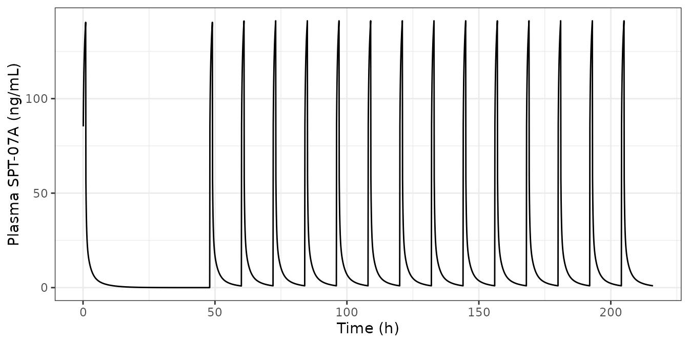
Replicates the human multiple-dose panel of Figure 6: 20 mg 1 h infusion, single dose on day 0 then q12h from 48 h.
Assumptions and deviations
Errata and source inconsistencies
1. PS is not reported anywhere and was
back-solved from a figure. Methods 2.5.1 states only that “PS
is the permeability-surface product, which was estimated by fitting this
value to the adipose concentration data in rats.” The fitted number
appears in no table, figure caption or text, and the article has no
supplementary material. It was recovered here by digitising the median
line of Figure 4J and solving for the PS that reproduces
it; the optimiser returns 0.499 mL/min against the authors’ evident
round value of 0.5, and at PS = 0.5 the model matches the
digitised curve to 5% on average and 10% at worst (table above). Because
PS governs distribution and not elimination, AUC
and clearance are mathematically independent of it – the
back-solve affects the adipose profile and the terminal phase only, and
none of the AUC or clearance validation above depends on it. The dog and
human values (17.0 and 140 mL/min) follow from Equation (13), which as
printed carries no exponent: the scaling is linear in
body weight, not allometric.
2. Table 3’s rat and dog predicted AUC cannot be reconciled with the paper’s own equations, and the profiles show the equations are right. The packaged implementation reproduces the human Table 3 predictions to within about 2% on Cmax, AUC and clearance at all three doses, and reproduces all eight of the paper’s Results 3.1.3 organ clearances exactly. For rats and dogs, however, the simulated AUC to infinity is systematically higher than the Table 3 predicted column – by the same factor at every dose level within a species, though a different factor between the two species – even though the predicted terminal half-lives match. Every number quoted in this section is computed below rather than transcribed, so it cannot drift out of step with the packaged models.
trapz <- function(t, conc) sum(diff(t) * (head(conc, -1) + tail(conc, -1)) / 2)

published_auc <- published |>
  dplyr::filter(PPTESTCD == "aucinf.obs") |>
  dplyr::select(species, dose_label, `Table 3 predicted` = PPORRES)

auc_window <- sims |>
  dplyr::filter(species != "human") |>
  dplyr::group_by(species, dose_label) |>
  dplyr::summarise(
    `Model AUC(0-inf)`  = trapz(time, Cc),
    `Model AUC(5-inf)`  = trapz(time[time >= 5], Cc[time >= 5]),
    .groups = "drop"
  ) |>
  dplyr::inner_join(published_auc, by = c("species", "dose_label")) |>
  dplyr::mutate(
    `Model / Table 3` = `Model AUC(0-inf)` / `Table 3 predicted`,
    `Table 3 within window range` =
      `Table 3 predicted` > `Model AUC(5-inf)` &
      `Table 3 predicted` < `Model AUC(0-inf)`
  )

auc_window |>
  dplyr::rename("Species" = species, "Dose" = dose_label) |>
  knitr::kable(
    digits = c(0, 0, 3, 3, 2, 3, 0),
    caption = paste(
    "Zhu 2024 Table 3's predicted animal AUC against the packaged model's AUC",
    "over two windows (mg*min/L). The ratio is constant across doses within a",
      "species -- as a linear model requires -- and Table 3 falls between the",
      "model's AUC from 5 min onward and its AUC to infinity in every arm."
    )
)| Species | Dose | Model AUC(0-inf) | Model AUC(5-inf) | Table 3 predicted | Model / Table 3 | Table 3 within window range |
|---|---|---|---|---|---|---|
| dog | 0.25 mg/kg | 6.302 | 3.070 | 3.60 | 1.750 | TRUE |
| dog | 0.5 mg/kg | 12.604 | 6.140 | 7.19 | 1.753 | TRUE |
| dog | 1 mg/kg | 25.207 | 12.279 | 14.40 | 1.750 | TRUE |
| rat | 0.5 mg/kg | 6.390 | 2.699 | 3.78 | 1.690 | TRUE |
| rat | 1 mg/kg | 12.779 | 5.397 | 7.56 | 1.690 | TRUE |
| rat | 2 mg/kg | 25.559 | 10.795 | 15.10 | 1.693 | TRUE |
# The overprediction must be a pure scale factor within each species (linear
# model), and the sampling-window explanation must actually hold in every arm.
ratio_spread <- auc_window |>
  dplyr::group_by(species) |>
  dplyr::summarise(spread = diff(range(`Model / Table 3`)), .groups = "drop")
stopifnot(
  nrow(auc_window) == 6L,
  all(auc_window$`Table 3 within window range`),
  max(ratio_spread$spread) < 0.01
)
The factor is 1.69-fold in the rat and 1.75-fold in the dog, while the predicted rat terminal half-life matches (59.0 min simulated versus 58.2 reported). Two further observations locate the problem in the Table 3 summary rather than in the model:
- The paper’s own stated systemic clearance for the rat – 75.0 mL/min/kg, Results 3.1.3 – agrees with the implemented equations, which give 78 mL/min/kg of plasma clearance (the small residual gap is the blood-to-plasma ratio plus sequential gut-to-liver extraction, neither of which the paper’s simple sum of organ clearances captures). Table 3’s predicted rat clearance of 129-132 mL/min/kg agrees with neither. The two numbers appear in the same paper and are mutually inconsistent, since AUC = Dose / CL.
- The rat plasma profile of Figure 4A agrees with the packaged model, so the figures support the printed equations; only the Table 3 AUC/CL column for the animal species does not.
fig4a <- tibble::tibble(
  time = c(30, 60, 90),
  `Digitised Fig 4A (ng/mL)` = c(107, 51.3, 29.8)   # rat plasma, 2 mg/kg
) |>
  dplyr::mutate(
    `Model (ng/mL)` = approx(rat2$time, rat2$Cc * 1000, xout = time)$y,
    `% diff` = 100 * (`Model (ng/mL)` - `Digitised Fig 4A (ng/mL)`) /
      `Digitised Fig 4A (ng/mL)`
  ) |>
  dplyr::rename("Time (min)" = time)

knitr::kable(fig4a, digits = c(0, 1, 1, 1),
caption = "Packaged rat model versus the digitised Figure 4A plasma profile (2 mg/kg IV bolus).")| Time (min) | Digitised Fig 4A (ng/mL) | Model (ng/mL) | % diff |
|---|---|---|---|
| 30 | 107.0 | 106.7 | -0.2 |
| 60 | 51.3 | 47.4 | -7.5 |
| 90 | 29.8 | 29.1 | -2.3 |
The most likely mechanism is the sampling window. Rats and dogs received an IV bolus with the first sample at 5 min, so an NCA that starts at the first observed concentration misses the steep 0-5 min distribution phase entirely; humans received a 1 h infusion, which has no such spike, and their numbers reconcile. Consistent with this, the paper’s rat and dog predicted AUC values sit between the model’s AUC to infinity and its AUC computed from 5 min onward in every arm – which the table above checks explicitly. Following the standing policy that a printed equation outranks a conflicting summary, the equations as printed are what is implemented; the rat and dog AUC rows of the comparison table above are starred for this reason and should not be read as an implementation defect.
3. Dog multiple-dose regimen is stated
inconsistently. Methods 2.3.3 says the dogs received 1 mg/kg qd
for 7 days; Table 3 labels the dog multiple-dose row 0.5 mg/kg and
reports the same predicted AUC (7.19) as its 0.5 mg/kg single-dose row.
The Table 3 label is self-consistent with the reported exposure and is
the one recorded in the model’s population metadata.
4. Blood-flow rounding. The dog tissue flows sum to 1121.46 mL/min against a printed cardiac output of 1120 (0.13%), and the human flows to 5600.33 against 5600 (0.006%). Both are reproduced as printed rather than reconciled, so the packaged values match Table 1 byte for byte. The rat closes exactly.
Assumptions
-
No IIV and no residual error. The paper’s 5th-95th
percentile bands come from 100 virtual subjects, but the magnitude and
distribution of the underlying parameter variability are never reported.
Rather than invent variances, both are omitted:
propSdisfixed(0)and no etas are declared. The packaged models are therefore deterministic typical-value simulators and cannot reproduce the prediction intervals in Figures 3-6, only the median lines. - Terminal half-life is window-dependent, and the window is assumed. The permeability-limited adipose compartment makes the model’s asymptotic terminal slope (rat 60, dog 139, human 217 min) much shallower than any observable half-life, so the comparison uses the final half of each species’ sampling window. Rat and dog windows come from Methods 2.3.1 and 2.3.3; the human window is assumed to be 12 h, since this paper does not report the clinical sampling schedule. The same rule is applied to all three species without per-arm tuning, and it recovers the paper’s predicted half-lives to within 5% in every species – but a reader who assumes a different clinical window will get a different human number, and none of the AUC, Cmax or clearance conclusions depends on this choice.
-
Observation compartment. The paper does not state
which blood pool its simulated plasma concentration is drawn from.
Venous plasma is used (
Cc <- c_venous / Rb), matching the sampling site for the dog (forearm vein) and human (venous) studies; the rat study sampled the femoral artery. Arterial and venous concentrations differ materially only during the first few minutes after a bolus. -
Blood versus plasma. Because
Kt:plis a tissue-to-plasma ratio while the perfusion terms carryKt:pl / Rb, the arterial, venous and adipose vascular states hold blood concentrations; the reported plasma concentration is obtained by dividing byRb. This follows directly from Equations (7)-(10) and is what makes the recomputed organ clearances match Results 3.1.3. -
Body weight is not a covariate. Organ volumes and
blood flows are the absolute Table 1 values for the reference animal
(0.25 kg rat, 8.5 kg beagle, 70 kg adult) and are not weight-scaled.
BWappears only in the per-kilogram intrinsic-clearance terms of Equations (14)-(16). Simulating a different body weight requires rescaling the volumes and flows as well, which the paper does not parameterise. -
MPPGL/MPPGK/MPPGIare not model parameters. These microsomal-protein scalars appear in Table 1 but act upstream, converting the measured in vitroCLint,uinto the whole-organCLint,in vivo,uvalues of Table 2 that the ODEs actually use. Only the Table 2 outputs are packaged. -
Compartment naming. The paper’s adipose
sub-compartments C1 and C2 are mapped to the registered canonicals
vp_adipose(vascular) andadipose(the tissue). The registeredis_adiposewas deliberately not used for C2, because theis_prefix denotes interstitial fluid, whereas for a small lipophilic monoterpene withKadipose:plasmaof 1.72-2.84 the extravascular space is predominantly intracellular lipid. The paper’s “rest of body” is the registeredother.