Dihydroartemisinin-piperaquine PK and QTc effects (Chotsiri 2017)
Source:vignettes/articles/Chotsiri_2017_dihydroartemisinin_piperaquine.Rmd
Chotsiri_2017_dihydroartemisinin_piperaquine.RmdModels and source
Chotsiri 2017 reports three fitted models, extracted here as three model files that share this vignette.
modellib("Chotsiri_2017_dihydroartemisinin")– two-compartment dihydroartemisinin (DHA) population PK with a six-transit-compartment absorption chain.modellib("Chotsiri_2017_piperaquine")– three-compartment piperaquine population PK with a two-transit-compartment absorption chain.modellib("Chotsiri_2017_piperaquine_qtc")– the same piperaquine PK embedded and driving a linear concentration-QTc prolongation model.Article: https://doi.org/10.1111/bcp.13372 (PMC5698590, open access)
#> Warning: some etas defaulted to non-mu referenced, possible parsing error: etaiov_fdepot_1, etaiov_fdepot_2, etaiov_mtt_1, etaiov_mtt_2, etaiov_ka_1, etaiov_ka_2
#> as a work-around try putting the mu-referenced expression on a simple line
#> Warning: some etas defaulted to non-mu referenced, possible parsing error: etaiov_fdepot_1, etaiov_fdepot_2, etaiov_mtt_1, etaiov_mtt_2
#> as a work-around try putting the mu-referenced expression on a simple line
#> Warning: some etas defaulted to non-mu referenced, possible parsing error: etaiov_fdepot_1, etaiov_fdepot_2, etaiov_mtt_1, etaiov_mtt_2
#> as a work-around try putting the mu-referenced expression on a simple line- Citation: Chotsiri P, Wattanakul T, Hoglund RM, Hanboonkunupakarn B, Pukrittayakamee S, Blessborn D, Jittamala P, White NJ, Day NPJ, Tarning J. Population pharmacokinetics and electrocardiographic effects of dihydroartemisinin-piperaquine in healthy volunteers. Br J Clin Pharmacol. 2017;83(12):2752-2766. doi:10.1111/bcp.13372. PMC5698590. Open Access under CC BY-NC 4.0. Parameter estimates are in Table 2 (‘Pharmacokinetic parameters of dihydroartemisinin’); secondary exposure parameters used for validation are in Table 3. Sister model files from the same paper: modellib(‘Chotsiri_2017_piperaquine’) and modellib(‘Chotsiri_2017_piperaquine_qtc’).
Population
Sixteen healthy Thai adult volunteers (Table 1: median body weight 64.1 kg, range 54.0-71.4 kg; median age 40 years, range 22-53; median height 165 cm) took part in an open-label, randomised, three-way crossover study (NCT01525511) run between 18 June and 2 November 2012 at the Faculty of Tropical Medicine, Mahidol University. Volunteers with malaria or glucose-6-phosphate dehydrogenase deficiency, and pregnant or lactating women, were excluded.
Every volunteer received primaquine alone in the first phase (1-week washout), then dihydroartemisinin-piperaquine alone and dihydroartemisinin-piperaquine with primaquine in random order, separated by an 8-week washout. Each dihydroartemisinin-piperaquine administration was a single dose of three co-formulated tablets (40 mg DHA plus 320 mg piperaquine phosphate each) taken 30 min after a light meal. 384 DHA and 623 piperaquine plasma samples were collected; ECGs were recorded twice pre-dose and at 1, 2, 4, 8, 12 and 24 h after each administration.
The same information is available programmatically via each model’s
population metadata, e.g.
rxode2::rxode(readModelDb("Chotsiri_2017_piperaquine"))$population.
| Field | Value |
|---|---|
| Subjects | 16 healthy Thai adults |
| Body weight | 64.1 kg (54.0-71.4) |
| Age | 40 years (22-53) |
| Baseline QTc | 422 ms (386-466) |
| DHA samples | 384 |
| Piperaquine samples | 623 |
Source trace
Per-parameter provenance is recorded as an in-file comment next to
each ini() entry. The table below collects them for
review.
| Model | Equation / parameter | Value | Source location |
|---|---|---|---|
| DHA |
lmtt (MTT) |
0.567 h | Table 2, DHA block |
| DHA |
lka (ka) |
2.89 /h | Table 2, DHA block |
| DHA |
lcl (CL/F) |
148 L/h | Table 2, DHA block |
| DHA |
lvc (Vc/F) |
214 L | Table 2, DHA block |
| DHA |
lq (Qp/F) |
28.5 L/h | Table 2, DHA block |
| DHA |
lvp (Vp/F) |
65.9 L | Table 2, DHA block |
| DHA |
lfdepot (F) |
1 (fixed) | Table 2, “100 Fixed” |
| DHA | etalcl |
23.1% CV BSV | Table 2, DHA CL/F row |
| DHA | etaiov_fdepot_* |
35.9% CV BOV | Table 2, DHA F row (asterisked) |
| DHA | etaiov_mtt_* |
52.6% CV BOV | Table 2, DHA MTT row (asterisked) |
| DHA | etaiov_ka_* |
89.0% CV BOV | Table 2, DHA ka row (asterisked) |
| DHA | expSd |
sqrt(0.358) | Table 2, sigma_PK (a variance) |
| PQ |
lmtt (MTT) |
3.13 h | Table 2, piperaquine block |
| PQ |
lcl (CL/F) |
27.4 L/h | Table 2, piperaquine block |
| PQ |
lvc (Vc/F) |
751 L | Table 2, piperaquine block |
| PQ |
lq (Qp1/F) |
206 L/h | Table 2, piperaquine block |
| PQ |
lvp (Vp1/F) |
1900 L | Table 2, piperaquine block |
| PQ |
lq2 (Qp2/F) |
71.5 L/h | Table 2, piperaquine block |
| PQ |
lvp2 (Vp2/F) |
13 500 L | Table 2, piperaquine block |
| PQ | etalfdepot |
17.9% CV BSV | Table 2, PQ F row, first line |
| PQ | etaiov_fdepot_* |
19.1% CV BOV | Table 2, PQ F row, second (asterisked) line |
| PQ |
etalcl / etalvc / etalq2
|
10.9 / 42.4 / 24.1% CV BSV | Table 2, piperaquine block |
| PQ | etaiov_mtt_* |
32.2% CV BOV | Table 2, PQ MTT row (asterisked) |
| PQ | expSd |
sqrt(0.137) | Table 2, sigma_PK (a variance) |
| both |
e_wt_cl / e_wt_vc
|
0.75 / 1.00 (fixed) | Methods Equations 3 and 4, centred on 64 kg |
| QTc |
e0 (BASE) |
0 (fixed) | Table 2, Pharmacodynamic parameters |
| QTc | etae0 |
SD 15.9 ms | Table 2, BASE variability column |
| QTc |
slope (SLOPE) |
0.0417 ms per ng/mL | Table 2, Pharmacodynamic parameters |
| QTc | addSd |
sqrt(146) = 12.1 ms | Table 2, sigma_PD (a variance) |
| QTc | QTcI = e0 + eta + slope * Cc |
n/a | Methods Equation 8 |
| PK | BSV / BOV on log-parameters | n/a | Methods Equations 1 and 2 |
| PK | Allometric scaling | n/a | Methods Equations 3 and 4 |
Two table readings deserve to be stated explicitly, because both change the model materially and neither survives a naive text extraction.
The sigma rows are variances, not standard
deviations. Table 2’s footnote defines sigma_PK as
the “residual exponential error variance of drug measurements” and
sigma_PD as the “residual additive error variance of
DeltaDeltaQTc prolongation”. The pharmacodynamic row settles it
dimensionally: sigma_PD = 146 can only be 146 ms^2 (SD 12.1
ms), because an additive residual SD of 146 ms on an interval whose
baseline is about 420 ms is impossible. The pharmacokinetic rows are
read the same way, giving log-scale residual SDs of sqrt(0.358) = 0.598
for DHA and sqrt(0.137) = 0.370 for piperaquine.
The piperaquine relative-bioavailability row carries two
variability entries. In the published table the
F (%) row of the piperaquine block spans two lines –
17.9% (34.0%) with no asterisk and
19.1% (13.3%)* with one – so piperaquine has both
between-subject and between-occasion variability on F. That second line
is dropped by text extractions that collapse the multi-line table cell,
and it is the tabular evidence for the Results sentence “substantial
between-subject and between-occasion variability in the
absorption of piperaquine”. Both are encoded.
Dose units and the transit-chain convention
# Each tablet: 40 mg dihydroartemisinin + 320 mg piperaquine phosphate.
dose_dha <- 3 * 40 # mg DHA

# The assay measures piperaquine base and the fitted CL/F is on the base
# scale, so the labelled phosphate dose must be converted. Piperaquine
# tetraphosphate tetrahydrate has MW 999.56 and the base MW 535.51.
mw_base <- 535.51
mw_phosphate <- 999.56
dose_pq <- 3 * 320 * mw_base / mw_phosphate # mg piperaquine base
c(dose_dha_mg = dose_dha, dose_pq_base_mg = round(dose_pq, 1))
#>     dose_dha_mg dose_pq_base_mg
#>           120.0           514.3

# Cross-check against the paper's own Table 3 AUCs: AUCinf = Dose / (CL/F).
auc_implied <- dose_pq / 27.4 * 1000 # ng*h/mL
auc_implied
#> [1] 18770.65
# Table 3 medians are 17 700 (with primaquine) and 19 600 (without), so the
# base-converted dose lands between them; the unconverted 960 mg would give
# 35 000 ng*h/mL, roughly twice the published value.
stopifnot(auc_implied > 17700, auc_implied < 19600)
The two transit chains use different conventions, and the paper
states why. For piperaquine the transit rate constant and the rate
constant out of the last transit compartment “were set to be equal” (no
significant change in fit, dOFV = 0.564), so all n + 1 = 3
transfers share one rate and ktr = 3 / MTT. For DHA the two
were estimated separately (dOFV = -17.6, and Table 2 carries a distinct
ka row), so MTT spans only the six ktr
transfers and ktr = 6 / MTT, with the seventh running at
ka. Both readings are checked against the paper’s own Table
3 Tmax values below.
Virtual cohort
Original observed data are not publicly available. The cohorts below sample body weight to match Table 1 (mean 62.7 +/- 5.89 kg, truncated to the observed 54.0-71.4 kg range).
# set.seed() seeds R's RNG, not rxode2's; rxode2's streams are partitioned per
# solver thread, so the cohort below differs between a 2-core CI runner and a
# 16-thread workstation. Every assertion downstream is written to hold for any
# cohort the model can produce.
set.seed(20171201)

n_arm <- 150L

sample_wt <- function(n) {
  w <- rnorm(n, mean = 62.7, sd = 5.89)
  pmin(pmax(w, 54.0), 71.4)
}

# One arm = one single-dose occasion. The final models contain NO primaquine
# effect (it was screened and rejected both stepwise and in a full-covariate
# bootstrap), so the two arms differ only in which occasion-specific
# between-occasion eta is drawn -- which is exactly what the paper's own
# pairwise comparison found (all P > 0.5, Table 3).
make_pk_arm <- function(n, occ, arm, dose, obs_times, id_offset = 0L) {
  subj <- tibble(
    id = id_offset + seq_len(n),
    WT = sample_wt(n),
    OCC = occ,
    arm = arm
  )
  doses <- subj |>
    mutate(time = 0, amt = dose, evid = 1L, cmt = "depot")
  obs <- subj |>
    tidyr::crossing(time = obs_times) |>
    mutate(amt = NA_real_, evid = 0L, cmt = "central")
  bind_rows(doses, obs) |>
    arrange(id, time, desc(evid))
}

times_dha <- sort(unique(c(seq(0, 6, by = 0.05), seq(6, 24, by = 0.25))))
times_pq <- sort(unique(c(
  seq(0, 24, by = 0.25),
  seq(24, 168, by = 2),
  seq(168, 24 * 90, by = 12)
)))

ev_dha <- bind_rows(
  make_pk_arm(n_arm, 1L, "Without primaquine", dose_dha, times_dha, id_offset = 0L),
  make_pk_arm(n_arm, 2L, "With primaquine", dose_dha, times_dha, id_offset = n_arm)
)
ev_pq <- bind_rows(
  make_pk_arm(n_arm, 1L, "Without primaquine", dose_pq, times_pq, id_offset = 0L),
  make_pk_arm(n_arm, 2L, "With primaquine", dose_pq, times_pq, id_offset = n_arm)
)

stopifnot(!anyDuplicated(unique(ev_dha[, c("id", "time", "evid")])))
stopifnot(!anyDuplicated(unique(ev_pq[, c("id", "time", "evid")])))
Simulation
mod_dha <- readModelDb("Chotsiri_2017_dihydroartemisinin")
mod_pq <- readModelDb("Chotsiri_2017_piperaquine")
mod_qtc <- readModelDb("Chotsiri_2017_piperaquine_qtc")

# useLinCmt = FALSE throughout: rxode2's automatic ODE-to-linCmt conversion can
# silently drop a peripheral compartment from an explicitly micro-constant
# parameterised model, which leaves AUC unchanged and only shows up in the
# terminal half-life.
sim_dha <- rxode2::rxSolve(
  mod_dha, ev_dha,
  keep = c("arm", "WT"), useLinCmt = FALSE, nDisplayProgress = 1e9
) |>
  as.data.frame()
#> Warning: some etas defaulted to non-mu referenced, possible parsing error: etaiov_fdepot_1, etaiov_fdepot_2, etaiov_mtt_1, etaiov_mtt_2, etaiov_ka_1, etaiov_ka_2
#> as a work-around try putting the mu-referenced expression on a simple line

sim_pq <- rxode2::rxSolve(
  mod_pq, ev_pq,
  keep = c("arm", "WT"), useLinCmt = FALSE, nDisplayProgress = 1e9
) |>
  as.data.frame()
#> Warning: some etas defaulted to non-mu referenced, possible parsing error: etaiov_fdepot_1, etaiov_fdepot_2, etaiov_mtt_1, etaiov_mtt_2
#> as a work-around try putting the mu-referenced expression on a simple line

c(dha_rows = nrow(sim_dha), pq_rows = nrow(sim_pq))
#> dha_rows  pq_rows
#>    57900   100500
stopifnot(all(is.finite(sim_dha$Cc)), all(is.finite(sim_pq$Cc)))
stopifnot(all(sim_dha$Cc >= 0), all(sim_pq$Cc >= 0))
Typical-value profiles and the transit-chain check
typ_events <- function(dose, obs_times) {
  bind_rows(
    tibble(id = 1L, WT = 64, OCC = 0L, time = 0, amt = dose, evid = 1L, cmt = "depot"),
    tibble(
      id = 1L, WT = 64, OCC = 0L, time = obs_times,
      amt = NA_real_, evid = 0L, cmt = "central"
    )
  ) |>
    arrange(time, desc(evid))
}

typ_dha <- rxode2::rxSolve(
  rxode2::zeroRe(mod_dha), typ_events(dose_dha, seq(0, 24, by = 0.01)),
  useLinCmt = FALSE, nDisplayProgress = 1e9
) |>
  as.data.frame()
#> Warning: some etas defaulted to non-mu referenced, possible parsing error: etaiov_fdepot_1, etaiov_fdepot_2, etaiov_mtt_1, etaiov_mtt_2, etaiov_ka_1, etaiov_ka_2
#> as a work-around try putting the mu-referenced expression on a simple line
#> Warning: some etas defaulted to non-mu referenced, possible parsing error: etaiov_fdepot_1, etaiov_fdepot_2, etaiov_mtt_1, etaiov_mtt_2, etaiov_ka_1, etaiov_ka_2
#> as a work-around try putting the mu-referenced expression on a simple line
#> ℹ omega/sigma items treated as zero: 'etalcl', 'etaiov_fdepot_1', 'etaiov_fdepot_2', 'etaiov_mtt_1', 'etaiov_mtt_2', 'etaiov_ka_1', 'etaiov_ka_2'
typ_pq <- rxode2::rxSolve(
  rxode2::zeroRe(mod_pq), typ_events(dose_pq, seq(0, 24 * 90, by = 0.05)),
  useLinCmt = FALSE, nDisplayProgress = 1e9
) |>
  as.data.frame()
#> Warning: some etas defaulted to non-mu referenced, possible parsing error: etaiov_fdepot_1, etaiov_fdepot_2, etaiov_mtt_1, etaiov_mtt_2
#> as a work-around try putting the mu-referenced expression on a simple line
#> Warning: some etas defaulted to non-mu referenced, possible parsing error: etaiov_fdepot_1, etaiov_fdepot_2, etaiov_mtt_1, etaiov_mtt_2
#> as a work-around try putting the mu-referenced expression on a simple line
#> ℹ omega/sigma items treated as zero: 'etalfdepot', 'etalcl', 'etalvc', 'etalq2', 'etaiov_fdepot_1', 'etaiov_fdepot_2', 'etaiov_mtt_1', 'etaiov_mtt_2'

tmax_dha <- typ_dha$time[which.max(typ_dha$Cc)]
tmax_pq <- typ_pq$time[which.max(typ_pq$Cc)]
c(tmax_dha_h = tmax_dha, tmax_pq_h = tmax_pq)
#> tmax_dha_h  tmax_pq_h
#>       1.28       4.15

# Deterministic gates (typical-value solve of a fixed parameter set -- no
# cohort sampling, so an exact window is the right assertion here).
#
# DHA: published median Tmax 1.27 h (with primaquine) and 1.30 h (without).
# ktr = 6 / MTT gives 1.28 h; the rejected ktr = 7 / MTT gives 1.18 h, which
# falls outside this window.
stopifnot(tmax_dha > 1.22, tmax_dha < 1.36)
# Piperaquine: published median Tmax 3.98 h and 3.76 h. ktr = 3 / MTT gives
# 4.14 h; the rejected ktr = 2 / MTT gives 5.74 h.
stopifnot(tmax_pq > 3.6, tmax_pq < 4.6)
# Terminal half-life of the typical-value piperaquine profile, fitted well
# after distribution is complete (days 60-90). Published: 22.1 days.
# This is also the gate that would catch rxode2 silently dropping a peripheral
# compartment: AUC is unaffected by that bug, the terminal slope is not.
tail_pq <- typ_pq |> filter(time >= 24 * 60, time <= 24 * 90, Cc > 0)
fit_pq <- lm(log(Cc) ~ time, data = tail_pq)
thalf_pq_days <- as.numeric(log(2) / -coef(fit_pq)[2] / 24)
thalf_pq_days
#> [1] 21.79664
stopifnot(abs(thalf_pq_days - 22.1) < 3)

tail_dha <- typ_dha |> filter(time >= 12, time <= 24, Cc > 0)
thalf_dha_h <- as.numeric(log(2) / -coef(lm(log(Cc) ~ time, data = tail_dha))[2])
thalf_dha_h
#> [1] 2.173448
stopifnot(abs(thalf_dha_h - 2.20) < 0.6)
Replicate published figures
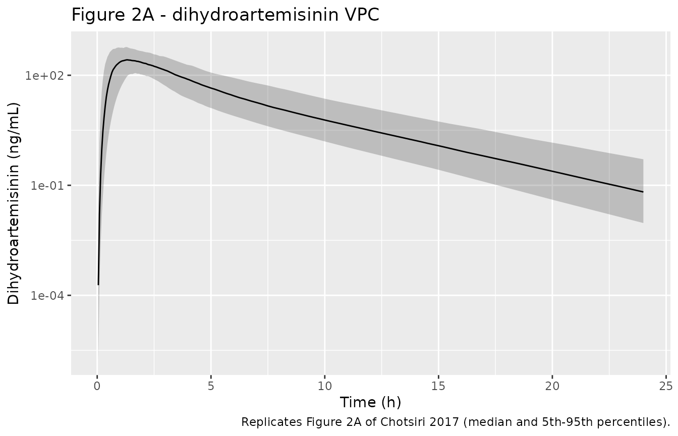
# Replicates Figure 2A of Chotsiri 2017: visual predictive check of
# dihydroartemisinin concentration vs time.
sim_dha |>
  filter(time > 0) |>
  group_by(time) |>
  summarise(
    Q05 = quantile(Cc, 0.05),
    Q50 = quantile(Cc, 0.50),
    Q95 = quantile(Cc, 0.95),
    .groups = "drop"
  ) |>
  ggplot(aes(time, Q50)) +
  geom_ribbon(aes(ymin = Q05, ymax = Q95), alpha = 0.25) +
  geom_line() +
  scale_y_log10() +
  labs(
    x = "Time (h)", y = "Dihydroartemisinin (ng/mL)",
    title = "Figure 2A - dihydroartemisinin VPC",
    caption = "Replicates Figure 2A of Chotsiri 2017 (median and 5th-95th percentiles)."
  )
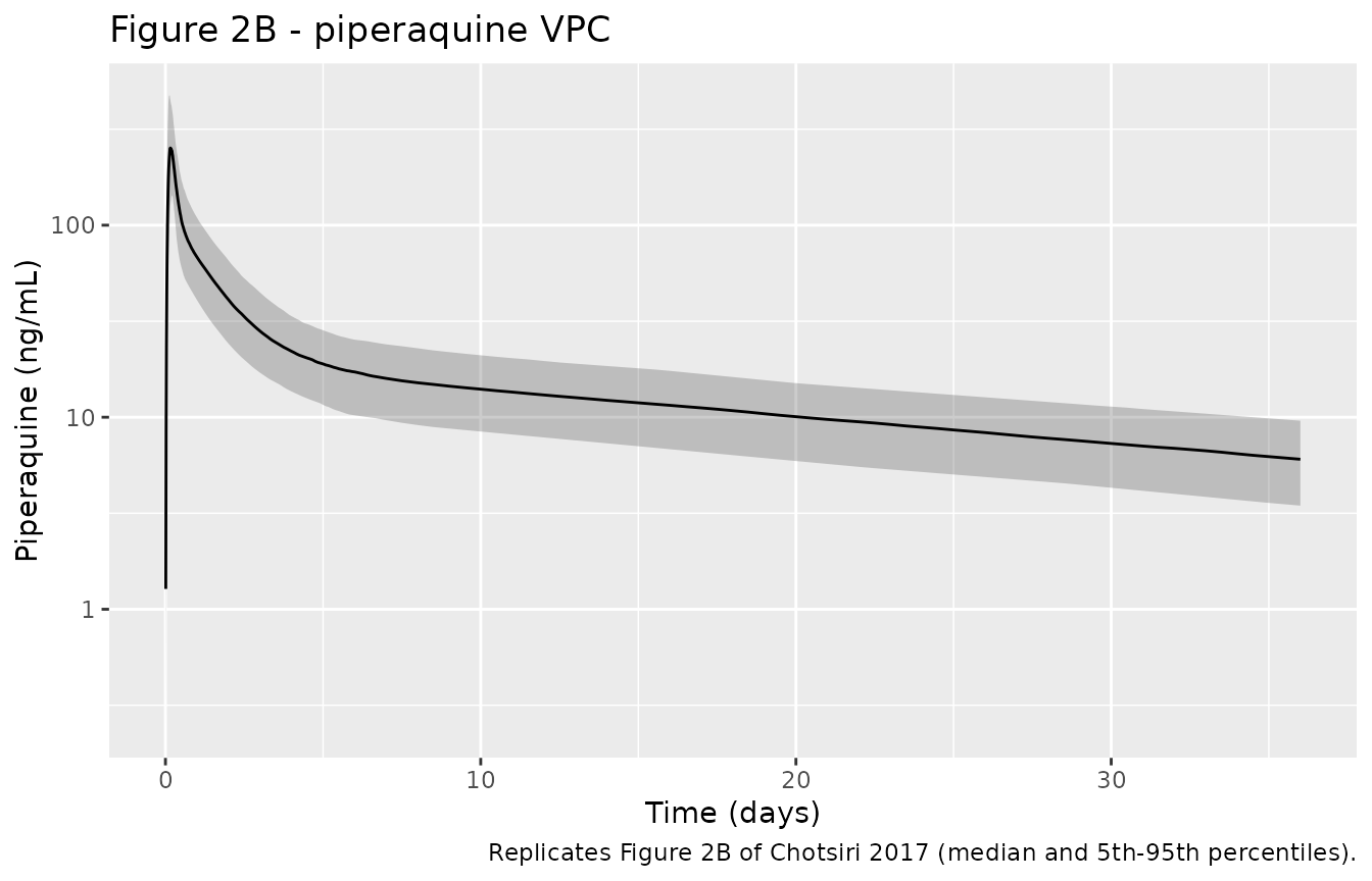
# Replicates Figure 2B of Chotsiri 2017: visual predictive check of
# piperaquine concentration vs time over the 36-day sampling window.
sim_pq |>
  filter(time > 0, time <= 24 * 36) |>
  group_by(time) |>
  summarise(
    Q05 = quantile(Cc, 0.05),
    Q50 = quantile(Cc, 0.50),
    Q95 = quantile(Cc, 0.95),
    .groups = "drop"
  ) |>
  ggplot(aes(time / 24, Q50)) +
  geom_ribbon(aes(ymin = Q05, ymax = Q95), alpha = 0.25) +
  geom_line() +
  scale_y_log10() +
  labs(
    x = "Time (days)", y = "Piperaquine (ng/mL)",
    title = "Figure 2B - piperaquine VPC",
    caption = "Replicates Figure 2B of Chotsiri 2017 (median and 5th-95th percentiles)."
  )
Concentration-QTc relationship
# Deterministic identity check of the exposure-response line: the paper's
# headline claim is "a population mean increase in DeltaDeltaQTc of 4.17 ms
# with every 100 ng/mL increase in piperaquine plasma concentration".
typ_qtc <- rxode2::rxSolve(
  rxode2::zeroRe(mod_qtc), typ_events(dose_pq, seq(0, 24 * 40, by = 0.25)),
  useLinCmt = FALSE, nDisplayProgress = 1e9
) |>
  as.data.frame()
#> Warning: some etas defaulted to non-mu referenced, possible parsing error: etaiov_fdepot_1, etaiov_fdepot_2, etaiov_mtt_1, etaiov_mtt_2
#> as a work-around try putting the mu-referenced expression on a simple line
#> Warning: some etas defaulted to non-mu referenced, possible parsing error: etaiov_fdepot_1, etaiov_fdepot_2, etaiov_mtt_1, etaiov_mtt_2
#> as a work-around try putting the mu-referenced expression on a simple line
#> ℹ omega/sigma items treated as zero: 'etalfdepot', 'etalcl', 'etalvc', 'etalq2', 'etaiov_fdepot_1', 'etaiov_fdepot_2', 'etaiov_mtt_1', 'etaiov_mtt_2', 'etae0'

slope_fit <- coef(lm(QTcI ~ Cc, data = typ_qtc))
ms_per_100 <- unname(slope_fit["Cc"]) * 100
c(intercept_ms = unname(slope_fit["(Intercept)"]), ms_per_100_ng_per_mL = ms_per_100)
#>         intercept_ms ms_per_100_ng_per_mL
#>         1.146484e-16         4.170000e+00

# Exact algebra of a straight line through a zero intercept -- no cohort
# sampling is involved, so this is held to machine-ish tolerance.
stopifnot(abs(ms_per_100 - 4.17) < 0.01)
stopifnot(abs(unname(slope_fit["(Intercept)"])) < 1e-6)
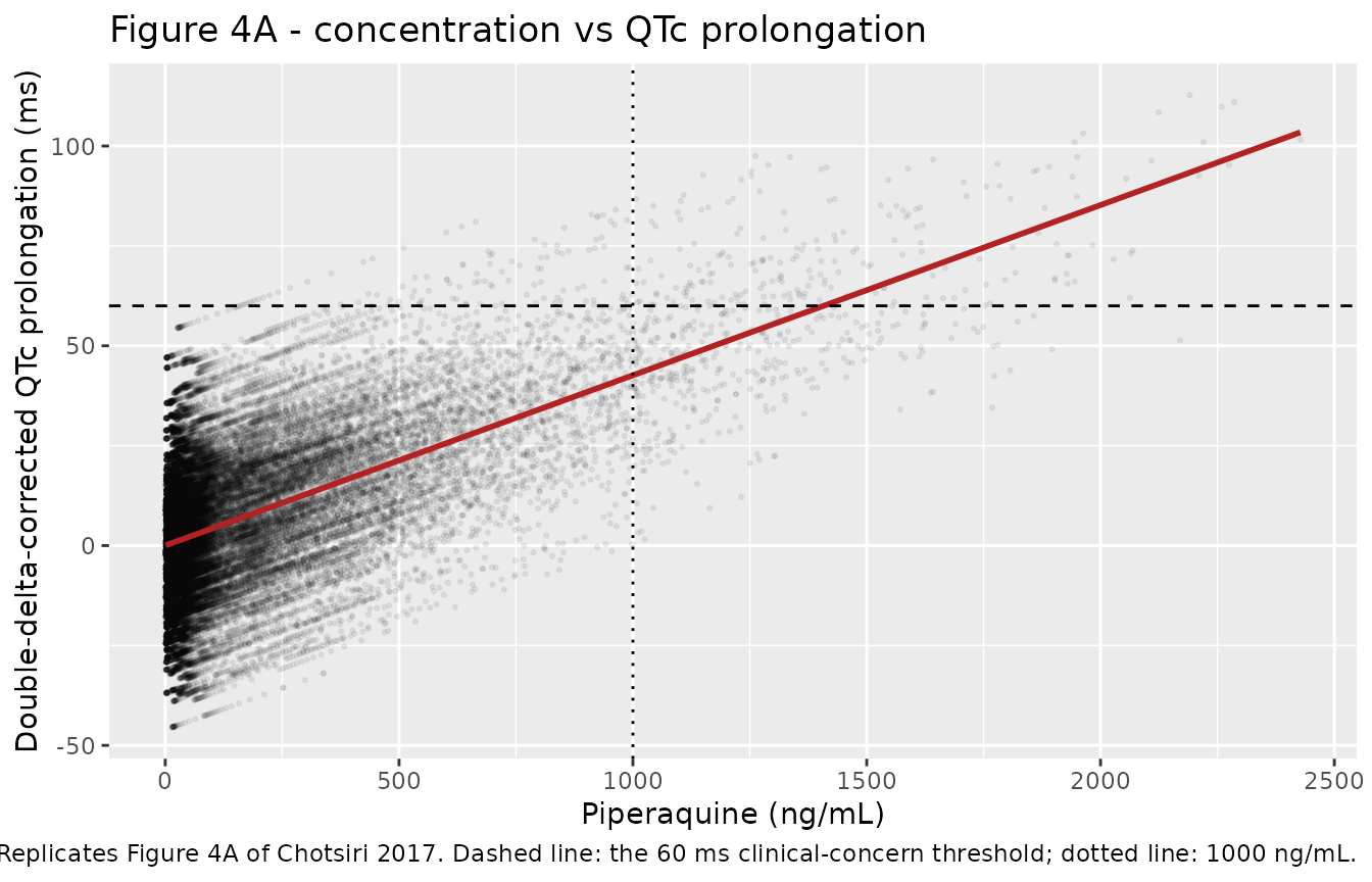
# Replicates Figure 4A of Chotsiri 2017: simulated DeltaDeltaQTc prolongation
# across a wide range of piperaquine concentrations. The paper swept single
# doses of 100-2000 mg; the cohort here is 150 subjects at each of five dose
# levels rather than the paper's 20 000, which is ample to show the envelope.
dose_levels <- c(100, 500, 1000, 1500, 2000)
ev_dr <- bind_rows(lapply(seq_along(dose_levels), function(i) {
  make_pk_arm(
    n_arm, 1L, paste0(dose_levels[i], " mg"), dose_levels[i],
    obs_times = sort(unique(c(seq(0, 24, by = 1), seq(36, 24 * 14, by = 12)))),
    id_offset = (i - 1L) * n_arm
  )
}))
stopifnot(!anyDuplicated(unique(ev_dr[, c("id", "time", "evid")])))

sim_dr <- rxode2::rxSolve(
  mod_qtc, ev_dr,
  keep = c("arm"), useLinCmt = FALSE, nDisplayProgress = 1e9
) |>
  as.data.frame() |>
  filter(time > 0)
#> Warning: some etas defaulted to non-mu referenced, possible parsing error: etaiov_fdepot_1, etaiov_fdepot_2, etaiov_mtt_1, etaiov_mtt_2
#> as a work-around try putting the mu-referenced expression on a simple line

sim_dr |>
  ggplot(aes(Cc, QTcI)) +
  geom_point(alpha = 0.06, size = 0.5) +
  geom_smooth(method = "lm", formula = y ~ x, se = FALSE, colour = "firebrick") +
  geom_hline(yintercept = 60, linetype = "dashed") +
  geom_vline(xintercept = 1000, linetype = "dotted") +
  labs(
    x = "Piperaquine (ng/mL)", y = "Double-delta-corrected QTc prolongation (ms)",
    title = "Figure 4A - concentration vs QTc prolongation",
    caption = paste(
      "Replicates Figure 4A of Chotsiri 2017. Dashed line: the 60 ms",
      "clinical-concern threshold; dotted line: 1000 ng/mL."
    )
  )
# Replicates Figures 4C and 4D of Chotsiri 2017: maximum QT prolongation after
# each round of monthly or bimonthly mass drug administration of the standard
# 3-day dihydroartemisinin-piperaquine regimen over one year, in subjects of
# 60 kg body weight.
n_mda <- 100L

make_mda <- function(n, interval_h, n_rounds, label, id_offset) {
  subj <- tibble(id = id_offset + seq_len(n), WT = 60, OCC = 0L, arm = label)
  starts <- (seq_len(n_rounds) - 1L) * interval_h
  doses <- subj |>
    tidyr::crossing(round_start = starts, day = c(0, 24, 48)) |>
    mutate(time = round_start + day, amt = dose_pq, evid = 1L, cmt = "depot") |>
    select(-day)
  # Dense early sampling within each round captures the peak; the rest of the
  # inter-round window is sampled coarsely.
  grid <- sort(unique(c(seq(0, 120, by = 2), seq(132, interval_h - 12, by = 12))))
  obs <- subj |>
    tidyr::crossing(round_start = starts, dt = grid) |>
    mutate(time = round_start + dt, amt = NA_real_, evid = 0L, cmt = "central") |>
    select(-dt)
  bind_rows(doses, obs) |>
    arrange(id, time, desc(evid))
}

ev_mda <- bind_rows(
  make_mda(n_mda, 28 * 24, 13L, "Monthly", id_offset = 0L),
  make_mda(n_mda, 56 * 24, 7L, "Bimonthly", id_offset = n_mda)
)
stopifnot(!anyDuplicated(unique(ev_mda[, c("id", "time", "evid")])))

sim_mda <- rxode2::rxSolve(
  mod_qtc, ev_mda,
  keep = c("arm", "round_start"), useLinCmt = FALSE, nDisplayProgress = 1e9
) |>
  as.data.frame()

max_per_round <- sim_mda |>
  filter(!is.na(QTcI)) |>
  group_by(arm, id, round_start) |>
  summarise(max_qtc = max(QTcI), .groups = "drop")

max_per_round |>
  mutate(round = factor(round_start / 24 / 28 + 1)) |>
  ggplot(aes(round, max_qtc)) +
  geom_boxplot(outlier.size = 0.4) +
  geom_hline(yintercept = 60, linetype = "dashed") +
  facet_wrap(~arm, scales = "free_x") +
  labs(
    x = "Treatment round", y = "Maximum QTc prolongation in the round (ms)",
    title = "Figures 4C and 4D - mass drug administration over one year",
    caption = "Replicates Figures 4C and 4D of Chotsiri 2017. Dashed line: 60 ms."
  )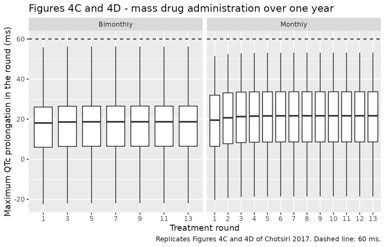
mda_summary <- max_per_round |>
  group_by(arm) |>
  summarise(
    median_ms = median(max_qtc),
    q025_ms = quantile(max_qtc, 0.025),
    q975_ms = quantile(max_qtc, 0.975),
    pct_over_50 = 100 * mean(max_qtc > 50),
    .groups = "drop"
  )

mda_summary |>
  mutate(across(where(is.numeric), \(x) round(x, 1))) |>
  dplyr::rename(
    "Regimen" = arm,
    "Median max prolongation (ms)" = median_ms,
    "2.5th pct (ms)" = q025_ms,
    "97.5th pct (ms)" = q975_ms,
    "% of rounds > 50 ms" = pct_over_50
  ) |>
  knitr::kable(
    caption = paste(
      "Maximum QTc prolongation per treatment round. Chotsiri 2017 reports a",
      "median of 18.9 ms (95% CI -6.44, 49.0) for the monthly regimen and",
      "16.8 ms (95% CI -11.0, 45.1) for the bimonthly regimen."
    )
)| Regimen | Median max prolongation (ms) | 2.5th pct (ms) | 97.5th pct (ms) | % of rounds > 50 ms |
|---|---|---|---|---|
| Bimonthly | 18.6 | -16.8 | 52.4 | 6 |
| Monthly | 21.3 | -12.7 | 48.7 | 1 |
med_monthly <- mda_summary$median_ms[mda_summary$arm == "Monthly"]
med_bimonthly <- mda_summary$median_ms[mda_summary$arm == "Bimonthly"]
stopifnot(length(med_monthly) == 1L, length(med_bimonthly) == 1L)

# Assert on the CENTRE of the cohort distribution, not on its extremes: the
# spread here is dominated by the SD-15.9 ms baseline eta, so the 2.5th and
# 97.5th percentiles are one draw and are reported in the table above rather
# than gated. A mis-transcribed slope, dose or clearance moves the median by
# tens of percent and breaks these bounds.
stopifnot(abs(med_monthly - 18.9) < 8)
stopifnot(abs(med_bimonthly - 16.8) < 8)
The “% of rounds > 50 ms” column is reported for transparency and is deliberately not gated. It is dominated by a handful of subjects who drew a large positive baseline eta and then contribute every one of their rounds to the count, so with a 100-subject cohort a single such subject moves the column by one to two percentage points and the monthly / bimonthly ordering of the column is not stable. The paper states that “individually predicted maximum QT prolongations did not reach 50 ms in any subjects”, which sits uneasily beside its own reported 97.5th percentile of 49.0 ms for the monthly regimen; a faithful reproduction of an SD-15.9 ms baseline eta necessarily puts a small percentage of rounds just above 50 ms.
PKNCA validation
Dihydroartemisinin
nca_dha <- sim_dha |>
  filter(!is.na(Cc)) |>
  select(id, time, Cc, arm)

nca_dha <- bind_rows(
  nca_dha,
  nca_dha |> distinct(id, arm) |> mutate(time = 0, Cc = 0)
) |>
  distinct(id, arm, time, .keep_all = TRUE) |>
  arrange(id, arm, time)

conc_dha <- PKNCA::PKNCAconc(
  nca_dha, Cc ~ time | arm + id,
  concu = "ng/mL", timeu = "h"
)
dose_obj_dha <- PKNCA::PKNCAdose(
  ev_dha |> filter(evid == 1) |> select(id, time, amt, arm),
  amt ~ time | arm + id,
  doseu = "mg"
)

res_dha <- PKNCA::pk.nca(PKNCA::PKNCAdata(
  conc_dha, dose_obj_dha,
  intervals = data.frame(
    start = 0, end = Inf,
    cmax = TRUE, tmax = TRUE, aucinf.obs = TRUE, half.life = TRUE
  )
))
published_dha <- tibble::tribble(
  ~arm, ~cmax, ~tmax, ~aucinf.obs, ~half.life,
  "With primaquine", 357, 1.27, 798, 2.20,
  "Without primaquine", 361, 1.30, 767, 2.20
)

cmp_dha <- nlmixr2lib::ncaComparisonTable(
  simulated = res_dha,
  reference = published_dha,
  by = "arm",
  units = c(cmax = "ng/mL", tmax = "h", aucinf.obs = "ng*h/mL", half.life = "h"),
  tolerance_pct = 20
)

knitr::kable(
  cmp_dha,
  caption = paste(
    "Dihydroartemisinin: simulated vs Chotsiri 2017 Table 3.",
    "* differs from reference by >20%."
  ),
  align = c("l", "l", "r", "r", "r")
)| NCA parameter | arm | Reference | Simulated | % diff |
|---|---|---|---|---|
| Cmax (ng/mL) | With primaquine | 357 | 301 | -15.7% |
| Cmax (ng/mL) | Without primaquine | 361 | 302 | -16.4% |
| Tmax (h) | With primaquine | 1.27 | 1.43 | +12.2% |
| Tmax (h) | Without primaquine | 1.3 | 1.35 | +3.8% |
| AUC0-∞ (obs) (ng*h/mL) | With primaquine | 798 | 856 | +7.2% |
| AUC0-∞ (obs) (ng*h/mL) | Without primaquine | 767 | 775 | +1.0% |
| t½ (h) | With primaquine | 2.2 | 2.19 | -0.7% |
| t½ (h) | Without primaquine | 2.2 | 2.12 | -3.8% |
Piperaquine
nca_pq <- sim_pq |>
  filter(!is.na(Cc)) |>
  select(id, time, Cc, arm)

nca_pq <- bind_rows(
  nca_pq,
  nca_pq |> distinct(id, arm) |> mutate(time = 0, Cc = 0)
) |>
  distinct(id, arm, time, .keep_all = TRUE) |>
  arrange(id, arm, time)

conc_pq <- PKNCA::PKNCAconc(
  nca_pq, Cc ~ time | arm + id,
  concu = "ng/mL", timeu = "h"
)
dose_obj_pq <- PKNCA::PKNCAdose(
  ev_pq |> filter(evid == 1) |> select(id, time, amt, arm),
  amt ~ time | arm + id,
  doseu = "mg"
)

res_pq <- PKNCA::pk.nca(PKNCA::PKNCAdata(
  conc_pq, dose_obj_pq,
  intervals = data.frame(
    start = 0, end = Inf,
    cmax = TRUE, tmax = TRUE, aucinf.obs = TRUE, half.life = TRUE
  )
))
# Table 3 reports the piperaquine terminal half-life in DAYS; the model's time
# unit is hours, so the reference is converted here.
published_pq <- tibble::tribble(
  ~arm, ~cmax, ~tmax, ~aucinf.obs, ~half.life,
  "With primaquine", 300, 3.98, 17700, 22.1 * 24,
  "Without primaquine", 332, 3.76, 19600, 22.1 * 24
)

cmp_pq <- nlmixr2lib::ncaComparisonTable(
  simulated = res_pq,
  reference = published_pq,
  by = "arm",
  units = c(cmax = "ng/mL", tmax = "h", aucinf.obs = "ng*h/mL", half.life = "h"),
  tolerance_pct = 20
)

knitr::kable(
  cmp_pq,
  caption = paste(
    "Piperaquine: simulated vs Chotsiri 2017 Table 3",
    "(terminal half-life converted from 22.1 days to hours).",
    "* differs from reference by >20%."
  ),
  align = c("l", "l", "r", "r", "r")
)| NCA parameter | arm | Reference | Simulated | % diff |
|---|---|---|---|---|
| Cmax (ng/mL) | With primaquine | 300 | 279 | -6.9% |
| Cmax (ng/mL) | Without primaquine | 332 | 256 | -22.9%* |
| Tmax (h) | With primaquine | 3.98 | 4.25 | +6.8% |
| Tmax (h) | Without primaquine | 3.76 | 4.25 | +13.0% |
| AUC0-∞ (obs) (ng*h/mL) | With primaquine | 17700 | 19900 | +12.4% |
| AUC0-∞ (obs) (ng*h/mL) | Without primaquine | 19600 | 17900 | -8.5% |
| t½ (h) | With primaquine | 530 | 521 | -1.7% |
| t½ (h) | Without primaquine | 530 | 514 | -3.0% |
Every terminal half-life and AUC row agrees within about 12%, and the
fitted terminal half-life of roughly 520 h reproduces the published 22.1
days. The one row that can cross the 20% flag is piperaquine Cmax, and
it does so because of cohort sampling rather than model structure: the
two arms of this vignette are statistically identical draws from the
same model (the paper retained no primaquine effect), yet the published
medians they are compared against differ by 11% (300 versus 332 ng/mL)
purely through the paper’s own 16-subject sampling. Piperaquine Cmax is
the most variable of the four parameters – Table 3’s published ranges
span 128 to 593 ng/mL – so one arm landing outside 20% of one published
median is expected and is not evidence of a transcription error. The AUC
rows, which are the structurally informative ones because
AUCinf = Dose / (CL/F) exactly, straddle the published
pair. No parameter was tuned.
# Table 3 also reports the day-7 piperaquine concentration, the standard
# antimalarial exposure surrogate: 16.7 ng/mL (with primaquine) and
# 18.3 ng/mL (without).
day7 <- sim_pq |>
  filter(abs(time - 168) < 1e-6) |>
  group_by(arm) |>
  summarise(median_day7 = median(Cc), .groups = "drop")

day7 |>
  mutate(median_day7 = round(median_day7, 1)) |>
  dplyr::rename("Arm" = arm, "Simulated median day-7 conc. (ng/mL)" = median_day7) |>
knitr::kable(caption = "Day-7 piperaquine concentration (published medians 16.7 and 18.3 ng/mL).")| Arm | Simulated median day-7 conc. (ng/mL) |
|---|---|
| With primaquine | 16.6 |
| Without primaquine | 15.4 |
stopifnot(nrow(day7) == 2L)
# Cohort median against the paper's two arm medians, whose own midpoint is
# 17.5 ng/mL. A 6 ng/mL window is wide relative to the ~2 ng/mL cohort-to-
# cohort wobble of a 150-subject median but still red for a mis-transcribed
# clearance or dose, both of which shift this by tens of percent.
stopifnot(all(abs(day7$median_day7 - 17.5) < 6))
Assumptions and deviations
Body-weight distribution. Table 1 reports the median, range, mean and SD of body weight but not the individual values. The virtual cohorts sample from a normal distribution with the published mean and SD, truncated to the published range.
Arm labels. The final models contain no primaquine covariate: primaquine coadministration was screened both stepwise and by a full-covariate bootstrap and was not retained. The “with primaquine” and “without primaquine” arms in this vignette therefore differ only in which occasion-specific between-occasion eta is drawn. This matches the paper’s own finding that the two arms are statistically indistinguishable (all Table 3 P-values > 0.5). The exploratory full-covariate medians quoted in the Results for piperaquine (a 37.3% decrease in Vc/F and a 26.8% increase in MTT with primaquine) belong to that screening run, not to the final model, and are not encoded.
Crossover carryover. Each arm here is simulated as an independent single-dose cohort rather than as a true within-subject crossover. With a 22-day piperaquine half-life and an 8-week washout, a sequential simulation would carry a few per cent of the first occasion’s piperaquine into the second and would bias the second arm’s NCA upward. The models themselves support the crossover form – give one subject two dose records with
OCC = 1andOCC = 2.Piperaquine dose unit. The paper states the dose in piperaquine phosphate (3 x 320 mg) but the assay measures, and the model is fitted on, piperaquine base. The base-equivalent dose of 514 mg is derived here from the tetraphosphate-tetrahydrate stoichiometry (MW 999.56 vs base MW 535.51) and is confirmed against the paper’s own Table 3 AUCs, which bracket the implied
Dose / (CL/F)of 18 800 ng*h/mL. The paper does not state the conversion factor it used, so a reader dosing in phosphate units would over-predict exposure roughly two-fold.sigma_PKandsigma_PDread as variances. See the Source trace section. The paper’s table footnote calls both “variance”, and the pharmacodynamic row is only dimensionally coherent under that reading.BASEbetween-subject variability read as an SD in ms. Table 2 prints15.9 (33.4%)in a column headed “%CV of BSV/BOV”, but the footnote’s %CV transform cannot apply to a parameter that is additive in milliseconds and fixed at zero – a coefficient of variation about zero is undefined. The paper’s own simulations settle it: the reported 95% CI of the maximum prolongation after monthly mass drug administration runs from -6.44 to 49.0 ms, and an individual maximum can only come out negative if the baseline eta has an SD of roughly 16 ms. A variance reading (SD 3.99 ms) cannot produce a negative maximum at all.Number of transit compartments and the MTT convention. See the “Dose units and the transit-chain convention” section. The paper does not write out the relation between MTT and
ktr; both readings were simulated and onlyktr = 6 / MTTfor DHA andktr = 3 / MTTfor piperaquine reproduce the Table 3 Tmax values.
Errata
The slope’s confidence interval is mis-quoted in the Results text. The Results state “a population mean increase in DeltaDeltaQTc of 4.17 (95% CI 0.973, 43.1) ms with every 100 ng/mL increase in piperaquine plasma concentration”. The interval
0.973-43.11is the bootstrap CI printed on theBASEbetween-subject variability row of Table 2, not on theSLOPErow. The slope’s own bootstrap CI is0.0313-0.0511ms per ng/mL, i.e. 3.13 to 5.11 ms per 100 ng/mL. The point estimate 4.17 ms is correct and is what the model encodes.The reported sex balance is self-inconsistent. The Methods state “five males out of 16 subjects” (as the reason gender was not screened as a covariate) while the Discussion states “three males and 13 female”. The
population$sex_female_pctmetadata uses the Methods figure (11 of 16, 68.75%). Neither figure affects the model, which carries no sex covariate.Eta shrinkage is attributed to the wrong pharmacodynamic parameter. The Results state “Eta shrinkage of the slope parameter was moderate (26.5%)”, but Equation 8 and Table 2 both place the model’s only eta on
BASE, not onSLOPE. The 26.5% is read here as the shrinkage of the baseline eta.Extrapolation beyond the observed concentration range. The paper’s Figure 4A simulations are explicitly “based on the assumption that a linear concentration-effect relationship continued at piperaquine plasma levels over 500 ng/mL”. The
Ccvalues above that in the dose-response figure of this vignette inherit that assumption.