Liposomal amphotericin B and miltefosine in PKDL (Chu 2026)
Source:vignettes/articles/Chu_2026_amphotericinB_liposomal.Rmd
Chu_2026_amphotericinB_liposomal.RmdModel and source
- Citation: Chu WY, Singh OP, Sundar S, Mondal D, Pandey K, Das P, Roseboom IC, Raja S, Torres A, Carrillo E, Huitema ADR, Alves F, Dorlo TPC. Bidirectional Interaction Between Liposomal Amphotericin B Pharmacokinetics and Parasite Dynamics in Patients With Post-Kala-Azar Dermal Leishmaniasis: Potential Implications for Optimal Dosing. Clin Pharmacol Ther. 2026;119(2):437-446. doi:10.1002/cpt.70124. Trial registration CTRI/2017/04/008421.
- Description: Joint population PK-PD model of liposomal amphotericin B (LAmB), oral miltefosine and skin parasite burden in 60 patients with post-kala-azar dermal leishmaniasis (PKDL) on the Indian subcontinent (Chu 2026), treated with LAmB 4 mg/kg on days 1, 4, 8, 11 and 15 alone or combined with 21 days of oral miltefosine. LAmB: two compartments (plasma and the mononuclear phagocyte system, MPS) with linear clearance from plasma and SATURABLE uptake into the MPS, kin * A_central * (1 - A_MPS / Bmax(t)), with first-order release kout. The MPS capacity Bmax(t) is a body-weight-scaled physiological baseline (10 mg at 45 kg, fixed) plus a disease component of 16 mg per log10 unit of the current parasite score, so the capacity falls as treatment clears the parasites and systemic LAmB exposure rises over the course of treatment. Miltefosine: two-compartment oral model allometrically scaled on fat-free mass (reference 40 kg), ka fixed, with relative bioavailability a power function (exponent fixed at -0.13) of the cumulative miltefosine dose in mg/kg. Parasite score (skin qPCR parasites/ug DNA times PKDL lesion score) is modelled on the log10 scale: the log10 score (baseline 4.7) decays first-order toward zero at a rate proportional to the LAmB amount in the MPS plus a rate proportional to the miltefosine plasma concentration, with no growth term, and is observed with additive error.
- Article: https://doi.org/10.1002/cpt.70124 (open access)
Chu et al. fitted a single joint PK-PD model to plasma total
amphotericin B, plasma miltefosine and a skin parasite score in patients
with post-kala-azar dermal leishmaniasis (PKDL). Its central feature is
a feedback loop: liposomal amphotericin B (LAmB) is taken up by the
mononuclear phagocyte system (MPS) with a capacity Bmax(t)
that grows with the parasite burden, the drug in the MPS clears the
parasites, and as the parasites clear the capacity shrinks so that more
drug stays in plasma. The model is packaged as one file because the
three parts were estimated jointly and are coupled through
Bmax(t) and the parasite kill terms.
Population
Sixty patients with PKDL from a phase II randomized trial in India (n = 50; two sites) and Bangladesh (n = 10), allocated 30/30 to LAmB monotherapy (AmBisome 4 mg/kg on days 1, 4, 8, 11 and 15; total 20 mg/kg) or the same LAmB regimen plus oral miltefosine twice daily for 21 days (Chu 2026 Methods and Table 1). Median age 22.5 years (IQR 15.8-36.3; 30% aged 18 or younger), 53.3% female, median body weight 45.5 kg (IQR 40.3-55), fat-free mass 39.2 kg (IQR 34.1-45) and BMI 19.0 kg/m^2. Baseline skin qPCR was a median 1050 parasites/ug DNA (IQR 156-5920) and the baseline PKDL lesion score a median 175 squares on the body map (IQR 75.5-262). The analysis used 646 amphotericin B and 143 miltefosine plasma samples and 177 parasite scores (baseline, day 30 and 3 months).
The same information is available programmatically via
readModelDb("Chu_2026_amphotericinB_liposomal")()$population.
Source trace
| Equation / parameter | Value | Source location |
|---|---|---|
d/dt(central), d/dt(mps)
|
saturable uptake
kin * A_central * (1 - A_MPS / Bmax(t)), release
kout * A_MPS, linear CL
|
Eq. 1; Figure 2 |
bmax_t |
Bmax,base * (WT/45) + Bmax,disease * A_parasite(t) |
Eq. 3; Table 2 footnote a |
d/dt(log10_parasites) |
-(lambda_LAmB * A_MPS + lambda_MF * C_MF) * A_parasite |
Eq. 4 |
f(depot_miltefosine) |
TVF * CumDose^COV |
Supplementary Methods S3, Equation S1 (day > 7 form) |
lcl |
log(0.3) L/h at 45 kg | Table 2 |
lvc |
log(3.1) L at 45 kg | Table 2 |
lkin_mps |
log(0.53) 1/h | Table 2 |
lkout_mps |
log(0.018) 1/h | Table 2 |
lbmax_mps |
log(10) mg at 45 kg, fixed | Table 2; Results |
lbmax_mps_disease |
log(16) mg per log10 unit | Table 2 |
e_wt_cl, e_wt_vc,
e_wt_bmax_mps
|
0.75, 1, 1 (fixed) | Table 2 footnote a; Results |
lcl_miltefosine |
log(0.086) L/h at FFM 40 kg | Table 2; Supplementary Results S1 |
lvc_miltefosine |
log(20) L at FFM 40 kg | Table 2 |
lq_miltefosine |
log(0.0012) L/h | Table 2 |
lvp_miltefosine |
log(1.9) L at FFM 40 kg | Table 2 |
lka_miltefosine |
log(0.225) 1/h, fixed | Table 2 footnote d; Supplementary Methods S3 |
lfdepot_miltefosine |
log(1), fixed | Supplementary Methods S3 |
e_dose_mf_cum_mgkg_fdepot |
-0.13, fixed | Table 2 footnote d; Supplementary Results S1 |
e_ffm_cl_miltefosine,
e_ffm_vc_vp_miltefosine
|
0.75, 1 (fixed) | Table 2 footnote c; Supplementary Methods S3 |
lslope_amphotericinb |
log(1.6e-4) 1/(mg h) | Table 2 |
lslope_miltefosine |
log(4.9e-5) L/(mg h) | Table 2 |
lrbase |
log(4.7) log10 units | Table 2 |
etalcl + etalvc |
43% and 32% CV, correlation 0.92 | Table 2 and footnote b |
etalkin_mps |
59% CV | Table 2 |
etalbmax_mps_disease |
40% CV | Table 2 |
etalcl_miltefosine |
19% CV | Table 2; Supplementary Results S1 |
etalslope_amphotericinb |
49% CV | Table 2 |
etalrbase |
350% CV | Table 2 |
propSd, addSd
|
0.22; 0.25 mg/L fixed | Table 2; Methods (LLOQ/2) |
propSd_miltefosine |
0.27 | Table 2 |
addSd_log10_parasites |
1.1 log10 units | Table 2 |
Every CV% is converted with omega^2 = log(1 + CV^2),
following the exponential BSV model stated in the Methods.
Event-table helper
All simulations share one builder. LAmB is a 2-hour IV infusion into
central; miltefosine is given twice daily into
depot_miltefosine. Observation rows sit on the
central ODE state and carry dvid = 1, because
the model declares three endpoints (Cc,
Cc_miltefosine, log10_parasites); every
observation row returns all three, plus mps and
bmax_t.
mod <- readModelDb("Chu_2026_amphotericinB_liposomal")

# `lamb_days` are 1-based treatment days; `mf_mg_day` = 0 gives monotherapy.
make_events <- function(id, wt, ffm, lamb_mgkg, lamb_days, mf_mg_day,
                        obs_times, mf_days = 21) {
  lamb <- tibble(
    id = id, time = 24 * (lamb_days - 1), amt = lamb_mgkg * wt,
    rate = lamb_mgkg * wt / 2, cmt = "central", evid = 1L, dvid = NA_integer_
  )
  mf <- if (mf_mg_day > 0) {
    tibble(
      id = id, time = sort(c(24 * (seq_len(mf_days) - 1), 24 * (seq_len(mf_days) - 1) + 12)),
      amt = mf_mg_day / 2, rate = 0, cmt = "depot_miltefosine", evid = 1L, dvid = NA_integer_
    )
  }
  obs <- tibble(
    id = id, time = obs_times, amt = 0, rate = 0, cmt = "central",
    evid = 0L, dvid = 1L
  )
  bind_rows(lamb, mf, obs) |>
    arrange(time, desc(evid)) |>
    mutate(
      WT = wt, FFM = ffm,
      # Running total of weight-normalized daily miltefosine doses including
      # the current day (Equation S1). It must stay positive, so monotherapy
      # rows carry a placeholder of 1; f(depot_miltefosine) is only ever
      # evaluated on miltefosine dose records.
      DOSE_MF_CUM_MGKG = if (mf_mg_day > 0) {
        pmin(floor(time / 24) + 1, mf_days) * mf_mg_day / wt
      } else {
        1
      }
    )
}
Typical patient: the PK-parasite feedback (Figure 3)
Figure 3 simulates a typical patient (45 kg, fat-free mass 40 kg, baseline log10 parasite score 4.7) on the trial regimen, alone or with miltefosine 150 mg/day.
typ_mod <- rxode2::zeroRe(mod)
obs_grid <- sort(unique(c(seq(0, 30 * 24, by = 0.25), seq(31 * 24, 90 * 24, by = 24))))
ev_typ <- bind_rows(
  make_events(1L, 45, 40, 4, c(1, 4, 8, 11, 15), 0, obs_grid) |> mutate(arm = "LAmB monotherapy"),
  make_events(2L, 45, 40, 4, c(1, 4, 8, 11, 15), 150, obs_grid) |> mutate(arm = "LAmB + miltefosine")
)
sim_typ <- rxode2::rxSolve(typ_mod, ev_typ, keep = "arm", returnType = "data.frame")
#> ℹ omega/sigma items treated as zero: 'etalcl', 'etalvc', 'etalkin_mps', 'etalbmax_mps_disease', 'etalcl_miltefosine', 'etalslope_amphotericinb', 'etalrbase'
#> Warning: multi-subject simulation without without 'omega'
The daily AUC of plasma amphotericin B (the bars in Figure 3) comes from PKNCA over consecutive 24-hour intervals:
conc_typ <- sim_typ |>
  filter(!is.na(Cc), time <= 30 * 24) |>
  select(id, arm, time, Cc)
dose_typ <- ev_typ |>
  filter(evid == 1, cmt == "central") |>
  select(id, arm, time, amt)
iv_daily <- data.frame(
  start = 24 * (0:29), end = 24 * (1:30), auclast = TRUE
)
nca_daily <- PKNCA::pk.nca(PKNCA::PKNCAdata(
  PKNCA::PKNCAconc(conc_typ, Cc ~ time | arm + id),
  PKNCA::PKNCAdose(dose_typ, amt ~ time | arm + id),
  intervals = iv_daily
))
daily_auc <- as.data.frame(nca_daily) |>
  filter(PPTESTCD == "auclast") |>
  transmute(arm, day = start / 24 + 1, auc_mgday = PPORRES / 24)
typ_long <- sim_typ |>
  filter(time <= 90 * 24) |>
  transmute(
    arm, day = time / 24,
    `Bmax in MPS (mg)` = bmax_t,
    `AmB in MPS (mg)` = mps,
    `Parasite score (log10) x 10` = 10 * log10_parasites
  ) |>
  pivot_longer(-c(arm, day), names_to = "quantity", values_to = "value")
ggplot() +
  geom_col(
    data = daily_auc, aes(x = day - 0.5, y = auc_mgday),
    fill = "#E6A65D", width = 0.9
  ) +
  geom_line(data = typ_long, aes(day, value, colour = quantity), linewidth = 0.8) +
  facet_wrap(~arm) +
  labs(
    x = "Time (days)", y = "Amount (mg), AUC (mg/L*day) or 10 x log10 score",
    colour = NULL,
    caption = "Replicates Figure 3 of Chu 2026. Bars: daily plasma AUC (mg/L*day)."
  ) +
  theme_bw() +
  theme(legend.position = "bottom")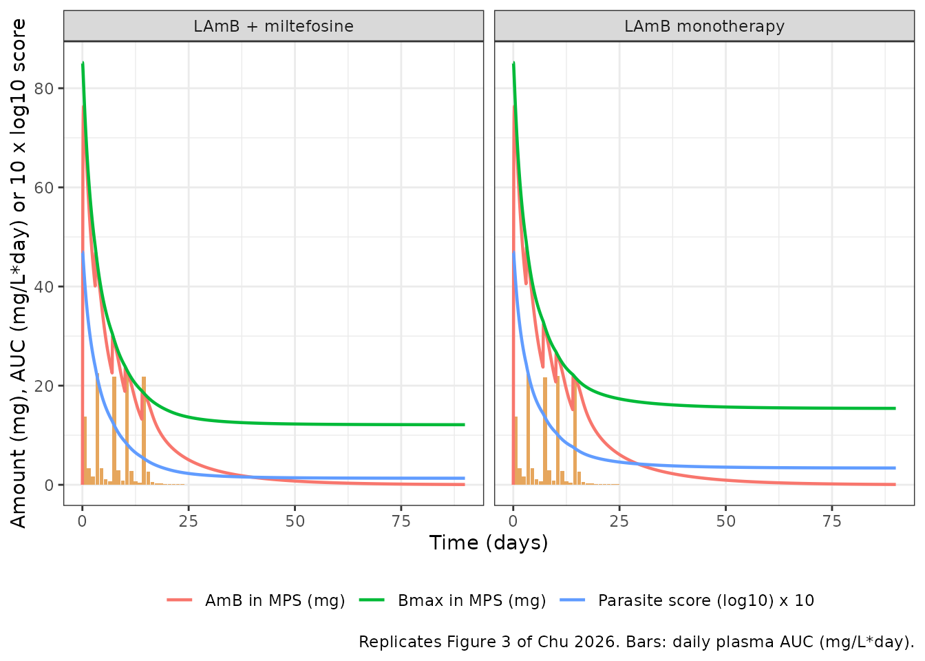
The paper states three numbers for this simulation. Under combination
therapy Bmax(t) on day 15 is down to 22% of its starting
value (Results: “a 22% decrease in Bmax by day 15”; Figure 3 shows the
curve falling from about 88 mg to about 20 mg, so the figure is the
remaining fraction, not the drop), and the day-15 plasma AUC0-24 is 54%
higher than on day 1. The plateaus after treatment are read from Figure
3.
bmax0 <- sim_typ |> filter(time == 0) |> select(arm, bmax0 = bmax_t)
bmax_d15 <- sim_typ |>
  filter(time == 14 * 24) |>
  left_join(bmax0, by = "arm") |>
  transmute(arm, bmax_d15 = bmax_t, frac_remaining = bmax_t / bmax0)
auc_ratio <- daily_auc |>
  filter(day %in% c(1, 15)) |>
  pivot_wider(names_from = day, values_from = auc_mgday, names_prefix = "day") |>
  mutate(ratio = day15 / day1)
plateau <- sim_typ |>
  filter(time == 90 * 24) |>
  select(arm, bmax_day90 = bmax_t, log10_parasites_day90 = log10_parasites)
fig3_tbl <- bmax_d15 |>
  left_join(auc_ratio, by = "arm") |>
  left_join(plateau, by = "arm")
fig3_tbl |>
  dplyr::rename(
    "Arm" = arm, "Bmax day 15 (mg)" = bmax_d15,
    "Bmax day 15 / day 1" = frac_remaining,
    "AUC0-24 day 1 (mg/L*day)" = day1, "AUC0-24 day 15 (mg/L*day)" = day15,
    "AUC ratio day 15 / day 1" = ratio, "Bmax day 90 (mg)" = bmax_day90,
    "log10 score day 90" = log10_parasites_day90
  ) |>
knitr::kable(digits = 3)| Arm | Bmax day 15 (mg) | Bmax day 15 / day 1 | AUC0-24 day 1 (mg/L*day) | AUC0-24 day 15 (mg/L*day) | AUC ratio day 15 / day 1 | Bmax day 90 (mg) | log10 score day 90 |
|---|---|---|---|---|---|---|---|
| LAmB monotherapy | 22.242 | 0.261 | 13.711 | 21.678 | 1.581 | 15.42 | 0.339 |
| LAmB + miltefosine | 18.936 | 0.222 | 13.721 | 21.824 | 1.591 | 12.12 | 0.132 |
combo <- fig3_tbl |> filter(arm == "LAmB + miltefosine")
mono <- fig3_tbl |> filter(arm == "LAmB monotherapy")
stopifnot(
  # Results: Bmax down to 22% of baseline by day 15 (combination).
  abs(combo$frac_remaining - 0.22) < 0.03,
  # Results: 54% higher systemic AUC0-24 on day 15 than on day 1.
  abs(combo$ratio / 1.54 - 1) < 0.10,
  # Figure 3 plateaus: Bmax about 15 mg (monotherapy) and 11 mg (combination).
  abs(mono$bmax_day90 - 15) < 2,
  abs(combo$bmax_day90 - 11) < 2
)
Alternative LAmB regimens (Figure 4)
Figure 4 compares four LAmB monotherapy regimens in the typical patient: the trial regimen, half the per-dose amount on the same schedule, a shortened schedule and a 10 mg/kg single dose. The comparison values were read from the figure at day 45 by the maintainers.
regimens <- tibble(
  regimen = c(
    "4 mg/kg x 5 over 15 days", "2 mg/kg x 5 over 15 days",
    "5 mg/kg x 4 over 7 days", "10 mg/kg single dose"
  ),
  mgkg = c(4, 2, 5, 10),
  days = list(c(1, 4, 8, 11, 15), c(1, 4, 8, 11, 15), c(1, 3, 5, 7), 1)
)
grid45 <- seq(0, 45 * 24, by = 0.25)
ev_reg <- bind_rows(lapply(seq_len(nrow(regimens)), function(i) {
  make_events(i, 45, 40, regimens$mgkg[i], regimens$days[[i]], 0, grid45) |>
    mutate(regimen = regimens$regimen[i])
}))
sim_reg <- rxode2::rxSolve(typ_mod, ev_reg, keep = "regimen", returnType = "data.frame") |>
  mutate(regimen = factor(regimen, levels = regimens$regimen))
#> ℹ omega/sigma items treated as zero: 'etalcl', 'etalvc', 'etalkin_mps', 'etalbmax_mps_disease', 'etalcl_miltefosine', 'etalslope_amphotericinb', 'etalrbase'
#> Warning: multi-subject simulation without without 'omega'
Cumulative AUCs to day 45, plasma (Cc) and MPS amount
(mps), by PKNCA:
dose_reg <- ev_reg |>
  filter(evid == 1) |>
  select(id, regimen, time, amt)
iv45 <- data.frame(start = 0, end = 45 * 24, auclast = TRUE)
nca45 <- function(col) {
  conc <- sim_reg |>
    filter(!is.na(.data[[col]])) |>
    transmute(id, regimen = as.character(regimen), time, conc = .data[[col]])
  res <- PKNCA::pk.nca(PKNCA::PKNCAdata(
    PKNCA::PKNCAconc(conc, conc ~ time | regimen + id),
    PKNCA::PKNCAdose(dose_reg, amt ~ time | regimen + id),
    intervals = iv45
  ))
  as.data.frame(res) |>
    filter(PPTESTCD == "auclast") |>
    mutate(PPORRES = PPORRES / 24)
}
sim45 <- bind_rows(
  nca45("Cc") |> mutate(quantity = "Plasma (mg/L*day)"),
  nca45("mps") |> mutate(quantity = "MPS (mg*day)")
) |>
  select(quantity, regimen, PPTESTCD, PPORRES)
ref45 <- tibble(
  quantity = rep(c("Plasma (mg/L*day)", "MPS (mg*day)"), each = 4),
  regimen = rep(regimens$regimen, 2),
  auclast = c(124, 62, 125, 62, 670, 655, 580, 515)
)
cmp45 <- ncaComparisonTable(sim45, ref45, by = c("quantity", "regimen"))
knitr::kable(cmp45, caption = "Cumulative AUC 0-45 days: simulated vs digitized Figure 4a-b.")| NCA parameter | quantity | regimen | Reference | Simulated | % diff |
|---|---|---|---|---|---|
| AUClast | Plasma (mg/L*day) | 4 mg/kg x 5 over 15 days | 124 | 125 | +0.7% |
| AUClast | Plasma (mg/L*day) | 2 mg/kg x 5 over 15 days | 62 | 62.3 | +0.5% |
| AUClast | Plasma (mg/L*day) | 5 mg/kg x 4 over 7 days | 125 | 125 | -0.1% |
| AUClast | Plasma (mg/L*day) | 10 mg/kg single dose | 62 | 62.4 | +0.6% |
| AUClast | MPS (mg*day) | 4 mg/kg x 5 over 15 days | 670 | 666 | -0.5% |
| AUClast | MPS (mg*day) | 2 mg/kg x 5 over 15 days | 655 | 650 | -0.7% |
| AUClast | MPS (mg*day) | 5 mg/kg x 4 over 7 days | 580 | 575 | -0.8% |
| AUClast | MPS (mg*day) | 10 mg/kg single dose | 515 | 509 | -1.1% |
stopifnot(all(abs(cmp45[["% diff"]] |> sub(pattern = "[*%]", replacement = "") |> as.numeric()) < 10))
sim_reg |>
  filter(time > 0) |>
  ggplot(aes(time / 24, log10_parasites, colour = regimen)) +
  geom_line(linewidth = 0.8) +
  labs(
    x = "Time (day)", y = "Parasite score (log10)", colour = NULL,
    caption = "Replicates Figure 4c of Chu 2026."
  ) +
  theme_bw() +
  theme(legend.position = "bottom") +
  guides(colour = guide_legend(nrow = 2))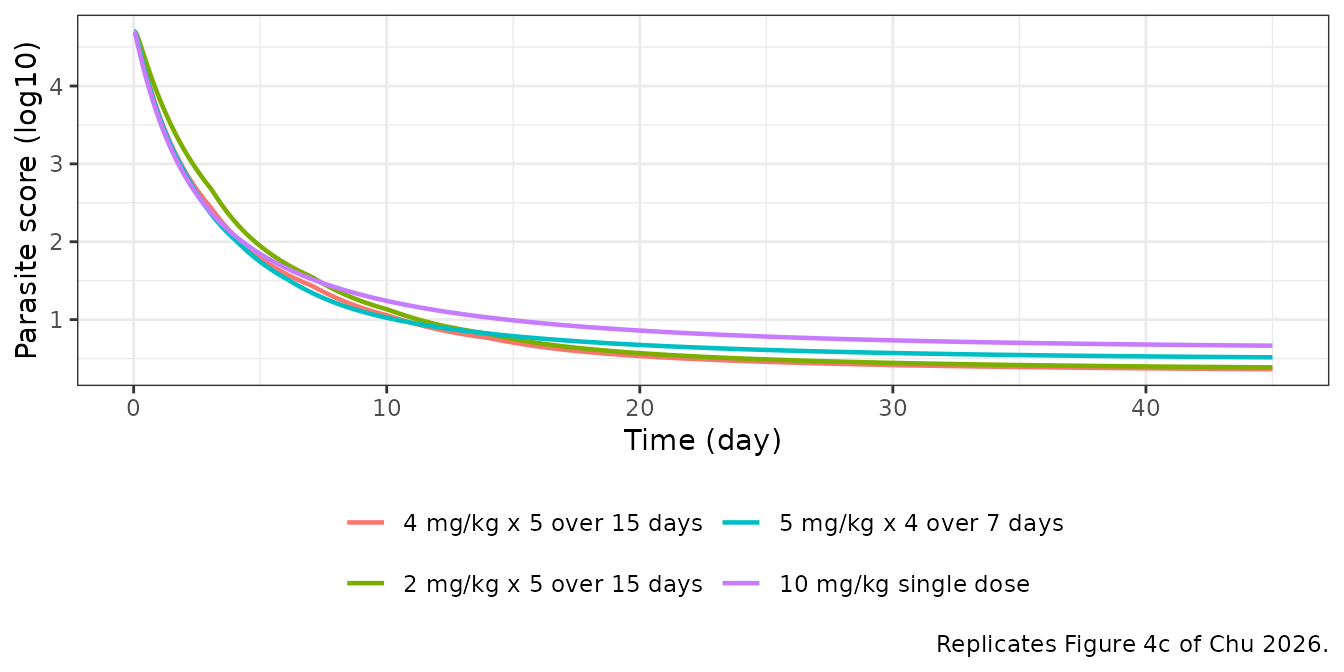
lp45 <- sim_reg |>
  filter(time == 45 * 24) |>
  select(regimen, sim = log10_parasites) |>
  mutate(digitized = c(0.35, 0.37, 0.48, 0.62))
knitr::kable(lp45, digits = 2, caption = "log10 parasite score on day 45 (digitized Figure 4c).")| regimen | sim | digitized |
|---|---|---|
| 4 mg/kg x 5 over 15 days | 0.36 | 0.35 |
| 2 mg/kg x 5 over 15 days | 0.39 | 0.37 |
| 5 mg/kg x 4 over 7 days | 0.52 | 0.48 |
| 10 mg/kg single dose | 0.67 | 0.62 |
The model reproduces the paper’s conclusion: halving the per-dose amount on the same five-dose schedule halves plasma exposure but leaves MPS exposure and parasite clearance close to the trial regimen, and it outperforms the same 10 mg/kg total given as a single dose.
Virtual trial cohort
A stochastic cohort of 100 subjects per arm, with body weight drawn
from a log-normal distribution matched to the Table 1 median and IQR.
The paper’s individual heights and sex are not available, so fat-free
mass is set to WT * 39.2 / 45.5 (the ratio of the Table 1
medians). Weights are kept above 30 kg so the miltefosine dose follows
the fixed 100 / 150 mg/day bands; the allometric miltefosine dosing of
patients of 30 kg or less is not reproduced.
rxode2::rxSetSeed(20261111)
set.seed(20261111)
n_arm <- 100
wts <- pmin(pmax(exp(rnorm(2 * n_arm, log(45.5), 0.23)), 30.5), 80)
obs_vpc <- sort(unique(c(
  seq(0, 24, by = 0.5), seq(14 * 24, 15 * 24, by = 0.5),
  24 * c(2:13, 16:30, 45, 60, 90)
)))
ev_vpc <- bind_rows(lapply(seq_len(2 * n_arm), function(i) {
  combo <- i > n_arm
  wt <- wts[i]
  mf <- if (!combo) 0 else if (wt >= 45) 150 else 100
  make_events(i, wt, wt * 39.2 / 45.5, 4, c(1, 4, 8, 11, 15), mf, obs_vpc) |>
    mutate(arm = if (combo) "LAmB + miltefosine" else "LAmB monotherapy")
}))
sim_vpc <- rxode2::rxSolve(mod, ev_vpc, keep = "arm", returnType = "data.frame")
Plasma amphotericin B after the first and last dose
pk_win <- sim_vpc |>
  filter(time <= 24 | (time >= 14 * 24 & time <= 15 * 24)) |>
  mutate(
    event = if_else(time <= 24, "First dose (day 1)", "Last dose (day 15)"),
    tad = if_else(time <= 24, time, time - 14 * 24)
  ) |>
  group_by(event, tad) |>
  summarise(
    p05 = quantile(Cc, 0.05), p50 = median(Cc), p95 = quantile(Cc, 0.95),
    .groups = "drop"
  )
ggplot(pk_win, aes(tad)) +
  geom_ribbon(aes(ymin = p05, ymax = p95), alpha = 0.25, fill = "steelblue") +
  geom_line(aes(y = p50), colour = "steelblue4") +
  facet_wrap(~event) +
  labs(
    x = "Time after dose (h)", y = "Plasma amphotericin B (mg/L)",
    caption = "Median and 90% interval; compare with the observed data in Figure 1a of Chu 2026."
  ) +
  theme_bw()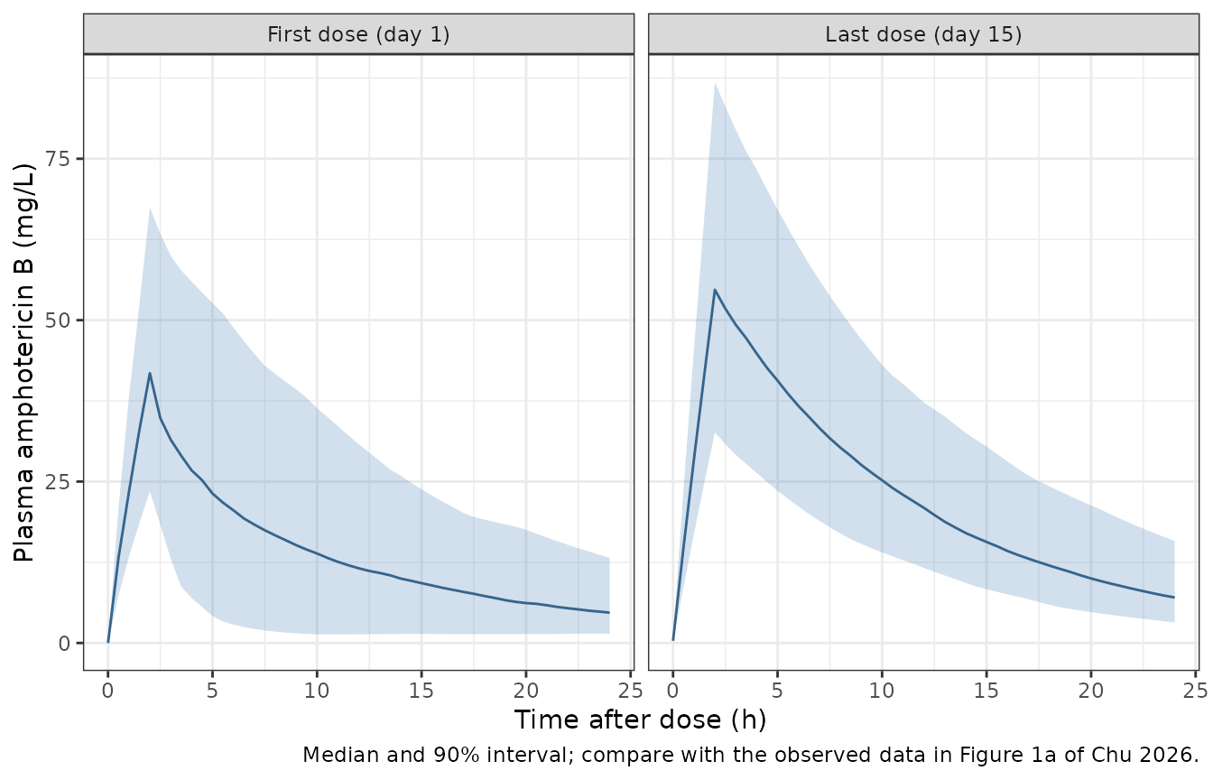
PKNCA on the first and last dosing interval:
conc_vpc <- sim_vpc |>
  filter(!is.na(Cc), time <= 15 * 24) |>
  select(id, arm, time, Cc)
dose_vpc <- ev_vpc |>
  filter(evid == 1, cmt == "central") |>
  select(id, arm, time, amt)
iv_vpc <- data.frame(
  start = c(0, 14 * 24), end = c(24, 15 * 24),
  cmax = TRUE, auclast = TRUE
)
nca_vpc <- PKNCA::pk.nca(PKNCA::PKNCAdata(
  PKNCA::PKNCAconc(conc_vpc, Cc ~ time | arm + id),
  PKNCA::PKNCAdose(dose_vpc, amt ~ time | arm + id),
  intervals = iv_vpc
))
nca_tbl <- as.data.frame(nca_vpc) |>
  mutate(day = if_else(start == 0, "day 1", "day 15")) |>
  group_by(arm, day, PPTESTCD) |>
  summarise(median = median(PPORRES), .groups = "drop") |>
  pivot_wider(names_from = PPTESTCD, values_from = median)
nca_tbl |>
  dplyr::rename(
    "Arm" = arm, "Dose" = day, "Cmax (mg/L)" = cmax,
    "AUC0-24 (mg*h/L)" = auclast
  ) |>
knitr::kable(digits = 1, caption = "Median simulated NCA parameters per dosing event.")| Arm | Dose | AUC0-24 (mg*h/L) | Cmax (mg/L) |
|---|---|---|---|
| LAmB + miltefosine | day 1 | 310.4 | 41.5 |
| LAmB + miltefosine | day 15 | 558.1 | 53.9 |
| LAmB monotherapy | day 1 | 344.6 | 41.9 |
| LAmB monotherapy | day 15 | 550.9 | 55.5 |
auc_ratio_ind <- as.data.frame(nca_vpc) |>
  filter(PPTESTCD == "auclast") |>
  select(id, arm, start, PPORRES) |>
  pivot_wider(names_from = start, values_from = PPORRES, names_prefix = "s") |>
  mutate(ratio = s336 / s0)
summary(auc_ratio_ind$ratio)
#>    Min. 1st Qu.  Median    Mean 3rd Qu.    Max.
#>   1.048   1.191   1.456   2.115   2.577  12.513
stopifnot(
  # Abstract: 'a median 54% increase in the systemic LAmB exposure (AUC0-24h)
  # by the end of treatment' (1.46 in the run documented here). The band is
  # wide because the median of 200 ratios with this spread moves by about
  # 0.08 between cohorts; losing the Bmax feedback would put it near 1.
  median(auc_ratio_ind$ratio) > 1.2,
  median(auc_ratio_ind$ratio) < 1.9
)
Plasma miltefosine and parasite score
mf_sum <- sim_vpc |>
  filter(arm == "LAmB + miltefosine", time %in% (24 * c(7, 14, 21, 28, 45, 60, 90))) |>
  group_by(day = time / 24) |>
  summarise(
    p05 = quantile(Cc_miltefosine, 0.05), p50 = median(Cc_miltefosine),
    p95 = quantile(Cc_miltefosine, 0.95), .groups = "drop"
  )
knitr::kable(mf_sum, digits = 1, caption = "Simulated plasma miltefosine (mg/L); compare Figure 1b of Chu 2026.")| day | p05 | p50 | p95 |
|---|---|---|---|
| 7 | 18.3 | 22.2 | 27.1 |
| 14 | 23.4 | 29.9 | 36.8 |
| 21 | 23.7 | 32.7 | 40.4 |
| 28 | 8.7 | 15.8 | 23.9 |
| 45 | 0.7 | 2.5 | 6.5 |
| 60 | 0.1 | 0.6 | 2.1 |
| 90 | 0.0 | 0.1 | 0.3 |
ps_sum <- sim_vpc |>
  filter(time %in% (24 * c(0, 30, 90))) |>
  group_by(arm, day = time / 24) |>
  summarise(
    p05 = quantile(log10_parasites, 0.05), p50 = median(log10_parasites),
    p95 = quantile(log10_parasites, 0.95), .groups = "drop"
  )
knitr::kable(ps_sum, digits = 2, caption = "Simulated individual log10 parasite score (no residual error).")| arm | day | p05 | p50 | p95 |
|---|---|---|---|---|
| LAmB + miltefosine | 0 | 0.58 | 4.10 | 49.80 |
| LAmB + miltefosine | 30 | 0.04 | 0.14 | 0.64 |
| LAmB + miltefosine | 90 | 0.02 | 0.10 | 0.52 |
| LAmB monotherapy | 0 | 0.32 | 4.46 | 78.08 |
| LAmB monotherapy | 30 | 0.05 | 0.32 | 1.29 |
| LAmB monotherapy | 90 | 0.04 | 0.25 | 1.01 |
The simulated miltefosine levels (5th-95th percentiles about 20-40 mg/L across days 7-21, falling after the last dose on day 21) match the range of Figure 1b. The parasite score shows how large the printed between-subject variability of the baseline is (see the next section): its 90% interval at baseline spans roughly 0.3-0.6 to 50-80 log10 units. The observed baselines in Figure 1c lie between about 1.5 and 8 log10 units, and the observed day-30 and 3-month scores (about 1 to 4.5 log10 units) sit well above the typical prediction of 0.1-0.4. The model reaches them only through that large baseline variability and the 1.1 log10 additive residual error.
Assumptions and deviations
-
Parasite score on the log10 scale. Eq. 4 is printed
as a first-order decline of
A_parasite. Eq. 3 multiplies the sameA_parasitebyBmax,disease, whose units are mg per log10(parasite score) (Table 2). The baseline is estimated as 4.7 log10 units, and the residual error is additive on the log10 scale. The state is therefore the log10 score itself, decaying exponentially toward 0. This reading reproduces the paper’s own simulations: Figure 3 plateaus and the 22%Bmaxfigure (above), and all twelve digitized day-45 values of Figure 4. Integrating Eq. 4 on the linear score instead leaves the typical patient near 2 log10 units at 3 months andBmaxat about 71% of its baseline on day 15, which contradicts Figure 3. -
“22% decrease in Bmax by day 15”. Figure 3 shows
Bmax(t)falling to about a quarter of its starting value by day 15, so the 22% is the fraction remaining, not the size of the drop. The model gives 22% remaining under combination therapy and 25% under monotherapy. -
Baseline BSV of 350% CV. Table 2 prints the
baseline log10 parasite score BSV as “350 (185-316)”: the point estimate
lies above its own SIR 95%
- The point estimate is encoded as printed
(
omega^2 = log(1 + 3.5^2)). With an exponential model on a log10-scale baseline, this produces implausibly wide individual baselines (see above), so treat stochastic parasite-score simulations with caution. Typical-value simulations are unaffected.
- The point estimate is encoded as printed
(
- lambda_LAmB units. Table 2 gives 1/(mg h) and the Results prose L/(mg h). Eq. 4 multiplies it by the MPS amount (mg), so 1/(mg h) is used.
-
Miltefosine bioavailability. Equation S1 has a
first-week malabsorption factor that was not supported in this cohort
(Supplementary Results S1), so only
F = CumDose^-0.13is applied.CumDosehas no normalizing value. The vignette builds it as the running sum of the weight-normalized daily dose including the current day. AtCumDose = 0the power function is infinite, so the column must be positive. Monotherapy subjects carry a placeholder of 1. - “More than 6-fold greater reduction in parasite score”. The Results compare the typical patient on combination therapy with monotherapy at 3 months. The model gives a remaining log10 score of 0.13 versus 0.34, a 2.6-fold ratio; Figure 3 shows about 0.05 versus 0.3. The miltefosine term is weaker here than in the paper’s figure. Setting bioavailability to 1 would close most of the gap, but it would also push day-21 miltefosine concentrations well above the Figure 1b observations. The equation and the values are kept as published.
- LAmB infusion duration is not stated; 2 hours (the usual AmBisome infusion) is assumed. Plasma AUC is insensitive to it.
- Fat-free mass is not derived from height and sex (not available); the virtual cohort scales it from body weight. Allometric miltefosine dosing for patients of 30 kg or less is not simulated.
- Region, lesion type, age, BMI and treatment arm were screened and
not retained (Results); they are documented in the model’s
covariatesDataExcluded.