Pirtobrutinib (Tian 2025)
Source:vignettes/articles/Tian_2025_pirtobrutinib.Rmd
Tian_2025_pirtobrutinib.RmdModel and source
- Citation: Tian DD, Hall SD, Chapman SC, Posada MM. (2025). Application of physiologically-based pharmacokinetic modeling to support drug labeling: prediction of CYP3A4-mediated pirtobrutinib-drug interactions. CPT Pharmacometrics Syst Pharmacol 14:2221-2231. doi:10.1002/psp4.70134.
- Description: Two-compartment oral pharmacokinetic reduction of the Simcyp minimal-PBPK-with-single-adjusting-compartment (SAC) model for the reversible BTK inhibitor pirtobrutinib in healthy adults (Tian 2025). The source model was built in the Simcyp Simulator version 19 and its whole-body mass-balance equations are not published, so the platform model itself cannot be encoded here. What IS fully reported is the pirtobrutinib compound layer, and it is sufficient to rebuild the disposition as an ordinary compartmental model: first-order absorption into a depot with a lag time, distribution between a systemic compartment and the SAC (the Simcyp kin / kout, encoded as the canonical k12 / k21), and first-order elimination from the systemic compartment. Systemic clearance is carried as the three components the paper’s disposition diagram prints separately, so a CYP3A4 perturbation can be applied to the CYP3A4-mediated arm alone: cl_3a4 (40% of systemic clearance), cl_other (non-CYP3A4 hepatic metabolism plus biliary excretion) and cl_renal. Hepatic availability is not a fitted constant but is derived inside the model from the well-stirred relationship the paper states as its Equation 2, so that oral bioavailability responds correctly when the CYP3A4 arm is changed. No parameter is fitted here: every value is either a Table 1 / Figure 2 / Data S3 input or an arithmetic consequence of one. The reduction reproduces the paper’s own predicted median tmax exactly after both a single 200 mg dose (2.94 h) and 200 mg once daily (2.72 h), and its predicted Cmax and AUC to within 8.3%; the residual offset is the difference between a typical-value individual and the geometric mean of the paper’s 100-subject virtual population (see the validation vignette). This is a typical-value simulation model: the source reports no estimated inter-individual variance components and no residual-error model, so there are no etas and propSd is fixed at zero. The drug-drug-interaction predictions that are the paper’s main contribution depend on proprietary Simcyp perpetrator compound files and on a CYP3A4 degradation rate constant that is never printed, so they are NOT reproducible mechanistically from this model; the vignette instead shows the closed-form CYP3A4-fraction envelope this reduction does support and compares it against the paper’s Figure 5.
- Article: https://doi.org/10.1002/psp4.70134
- Open-access full text and supplement: https://www.ncbi.nlm.nih.gov/pmc/articles/PMC12706395/
- Supplement Data S1 (figures), Data S2 (Supplementary Materials 1-5,
Tables S1-S14), Data S3 (Simcyp input sheet,
.xlsx)
What this model is, and what it is not
Tian 2025 built a minimal PBPK model with a single adjusting compartment (SAC) for pirtobrutinib in the Simcyp Simulator version 19, and used it to predict drug-drug interactions (DDIs) with CYP3A4 inhibitors and inducers in support of the product label.
Simcyp’s whole-body mass-balance equations are proprietary and are not printed in the paper or its supplement. The six numbered equations in the main text are all input-derivation formulae (hepatic clearance, hepatic availability, biliary clearance, the intestinal-availability back-calculation, and the fraction absorbed), never the disposition ODEs. The platform model therefore cannot be encoded as published.
What is fully reported is the pirtobrutinib compound layer, and it is unusually complete:
- Table 1 gives the physicochemical, absorption, distribution and elimination inputs.
-
Figure 2 (the proposed disposition diagram) prints
the entire clearance decomposition –
CL,CL_H,CL_hepatic metabolism,CL_bile,CL_R,f_m,CYP3A4,f_m,other,f_e,bile,f_e,urine– together withFa,Fg,Fh,FandVss. -
Data S3, the Simcyp input sheet itself, reports the
SAC rate constants
kinandkoutto full double precision alongside the inter-compartmental clearanceQ.
Because kin = Q / V_systemic and
kout = Q / V_SAC, those three numbers pin the systemic
volume in absolute litres, so this reduction needs no assumed
reference body weight anywhere. Every parameter in the packaged
model is either a printed input or a one-step arithmetic consequence of
printed inputs; nothing is fitted here and nothing is imported from a
Simcyp population file.
What is not reproducible:
- The time-dependent inhibition (TDI) of CYP3A4 by
pirtobrutinib itself. Table 1 reports
K_I= 4.70 uM and the fittedk_inact= 0.056 1/h, but the autoinhibition ODE also needs the CYP3A4 degradation rate constantk_deg, which is a Simcyp database value and is never printed. This model is therefore the linear pirtobrutinib model, and is validated against the paper’s own “without TDI” predictions (Table 2, and the “reversible inhibition” row of Table S9), which the paper reports separately for exactly this comparison. - The perpetrator models (itraconazole, hydroxyitraconazole, ritonavir, ketoconazole, clarithromycin, diltiazem, fluconazole, verapamil, rifampin, efavirenz, bosentan, modafinil, midazolam). These are proprietary Simcyp compound files or literature PBPK models, so the DDI simulations cannot be run mechanistically. The final section instead exercises the closed-form CYP3A4-fraction envelope that this reduction does support, and shows it reproduces the paper’s Figure 5 predictions.
- Population variability. Data S3 prints 30% input CVs on
ka, lag time,Q_gut, the additional HLMCLintand the biliaryCLint, but the percent-CV figures in Table 2 are dominated by liver weight and CYP3A4 abundance drawn from Simcyp population files. No variance is invented here;propSdis fixed at zero and the model is a deterministic typical-value simulation.
Population
pop <- rxode2::rxode(readModelDb("Tian_2025_pirtobrutinib"))$meta$population
str(pop, max.level = 1)
#> List of 11
#>  $ species       : chr "human"
#>  $ n_subjects    : int 100
#>  $ n_studies     : int 9
#>  $ age_range     : chr "20-55 years for the 200 mg once-daily simulation (Data S3); 19-55 years for the single-dose simulation (Table S4)"
#>  $ weight_median : chr "not reported; the Simcyp Sim-Healthy Volunteers default distribution was used"
#>  $ sex_female_pct: num 25
#>  $ disease_state : chr "Healthy adult volunteers, fasted, CYP3A5 genotype unrestricted for the pirtobrutinib-alone simulations."
#>  $ dose_range    : chr "Single oral dose of 200 mg, and 200 mg once daily for 13 doses (Data S3)."
#>  $ regions       : chr "Simcyp Sim-Healthy Volunteers virtual population (Data S3)."
#>  $ studies       : chr "Nine clinical pharmacology studies supplied the observations and the compound-layer inputs (Supplemental Materi"| __truncated__
#>  $ notes         : chr "n_subjects records the 100 virtual subjects (10 trials of 10) Data S3 simulated for pirtobrutinib alone, becaus"| __truncated__
All simulations in Tian 2025 were run in healthy volunteers using the
Simcyp Sim-Healthy Volunteers population in PK/PD Profiles
mode. For pirtobrutinib dosed alone, Data S3 records 10 trials of 10
subjects (100 virtual subjects), age 20-55 years, 25% female, fasted,
200 mg once daily for 13 doses. The single-dose simulation used age
19-55 years and 18% female (Table S4), matched to the contributing
clinical studies.
Nine clinical pharmacology studies supplied the observations and the compound-layer inputs (Supplemental Material 1). The absolute bioavailability study (n = 5 healthy males, NCT06180954) is the anchor for this reduction: it supplies the intravenous systemic clearance, the renal clearance, the steady-state volume and the absolute oral bioavailability.
The reduction, step by step
Every derived number in the packaged model is reproduced below from printed source values, so the arithmetic can be checked independently of the model file.
# --- Data S3 (Simcyp input sheet), Distribution block -----------------
sacKin  <- 0.12402043422142926  # "SAC kin (1/h)"
sacKout <- 0.2594761264470896   # "SAC kout (1/h)"
sacQ    <- 3.56                 # "SAC Q (L/h)"; Table 1 Q = 3.56 L/h

vcDer  <- sacQ / sacKin   # kin  = Q / V_systemic
vsacDer<- sacQ / sacKout  # kout = Q / V_SAC

# Table 1 gives V_SAC = 0.17 L/kg, so the implied body weight of the
# Simcyp population representative is a consistency check on the reading:
bwImplied <- vsacDer / 0.17

# --- Figure 2 (proposed disposition diagram) --------------------------
clTotal <- 1.69   # systemic plasma clearance (L/h)
clRen   <- 0.12   # CL_R
clHepMet<- 1.33   # CL_hepatic metabolism
clBile  <- 0.24   # CL_bile
fmCyp3a4<- 0.40   # f_m,CYP3A4

cl3a4   <- fmCyp3a4 * clTotal          # CYP3A4-mediated arm
clOther <- (clHepMet - cl3a4) + clBile # non-CYP3A4 hepatic + biliary

# --- Equations 1, 2 and 6 --------------------------------------------
bp <- 0.79; qh <- 90            # Table 1 B:P; main text Q_H = 90 L/h
clH   <- cl3a4 + clOther        # Equation 1: CL_H = CL - CL_R
fhDer <- 1 - clH / (bp * qh)    # Equation 2
fgut  <- 0.96                   # Equation 5 (Fg)
fabs  <- 0.86 / (fgut * fhDer)  # Equation 6, from measured F = 0.86

data.frame(
  Quantity = c("vc = Q / kin (L)", "V_SAC = Q / kout (L)",
               "implied body weight (kg)", "cl_3a4 (L/h)", "cl_other (L/h)",
               "CL_H = cl_3a4 + cl_other (L/h)", "CL = CL_H + CL_R (L/h)",
               "Fh (Equation 2)", "Fa (Equation 6)", "F = Fa x Fg x Fh"),
  Derived = c(vcDer, vsacDer, bwImplied, cl3a4, clOther, clH,
              clH + clRen, fhDer, fabs, fabs * fgut * fhDer),
  Printed = c(NA, NA, NA, NA, NA, 1.57, 1.69, 0.98, 0.91, 0.86),
  Source = c("Data S3 / Table 1", "Data S3 / Table 1",
             "cross-check vs Table 1 V_SAC 0.17 L/kg", "Figure 2",
             "Figure 2", "Figure 2", "Figure 2", "Figure 2", "Table 1",
             "Figure 2")
) |>
  dplyr::mutate(Derived = signif(Derived, 6)) |>
knitr::kable(caption = "Derived reduction inputs against the values Tian 2025 prints.")| Quantity | Derived | Printed | Source |
|---|---|---|---|
| vc = Q / kin (L) | 28.704900 | NA | Data S3 / Table 1 |
| V_SAC = Q / kout (L) | 13.720000 | NA | Data S3 / Table 1 |
| implied body weight (kg) | 80.705600 | NA | cross-check vs Table 1 V_SAC 0.17 L/kg |
| cl_3a4 (L/h) | 0.676000 | NA | Figure 2 |
| cl_other (L/h) | 0.894000 | NA | Figure 2 |
| CL_H = cl_3a4 + cl_other (L/h) | 1.570000 | 1.57 | Figure 2 |
| CL = CL_H + CL_R (L/h) | 1.690000 | 1.69 | Figure 2 |
| Fh (Equation 2) | 0.977918 | 0.98 | Figure 2 |
| Fa (Equation 6) | 0.916061 | 0.91 | Table 1 |
| F = Fa x Fg x Fh | 0.860000 | 0.86 | Figure 2 |
The clearance components sum back to the printed total exactly, and
the Equation 2 / Equation 6 chain returns the printed Fh =
0.98 and F = 0.86. The V_SAC reading also
reproduces a body weight of 80.7 kg for the Simcyp population
representative, which is what confirms that kin is
Q / V_systemic rather than the reverse.
The paper’s Equations 4 and 5 round-trip as well. Equation 4
approximates the pirtobrutinib Cmax ratio from the
intestinal availability Fg and the fraction of intestinal
CYP3A4 activity remaining under itraconazole, X = 0.009
(Table S3):
xItra <- 0.009
c(`Eq 4: Cmax ratio from Fg = 0.96 and X = 0.009` = 1 / (fgut + (1 - fgut) * xItra),
  `Eq 5: Fg back from the observed +4% Cmax rise` = (1 / 1.04 - xItra) / (1 - xItra))
#> Eq 4: Cmax ratio from Fg = 0.96 and X = 0.009
#>                                     1.0412762
#> Eq 5: Fg back from the observed +4% Cmax rise
#>                                     0.9611892
Equation 4 returns a 4.1% Cmax rise against the observed
4%, and Equation 5 returns Fg = 0.961 against the printed
0.96.
Source trace
| Item | Source |
|---|---|
| ka = 0.82 1/h | Table 1, fitted to observed tmax/Cmax; Data S3 row ‘ka (1/h)’ |
| t_lag = 0.25 h | Table 1; Data S3 row ‘lag time (h)’ |
| cl_3a4 = 0.676 L/h | Figure 2: f_m,CYP3A4 (0.40) x CL (1.69 L/h) |
| cl_other = 0.894 L/h | Figure 2: (CL_hepatic metabolism 1.33 - 0.676) + CL_bile 0.24 |
| cl_renal = 0.12 L/h | Table 1 and Figure 2, measured from the intravenous dose |
| vc = 28.7049 L | Data S3: SAC Q (3.56) / SAC kin (0.12402043422142926) |
| k12 = 0.1240204 1/h | Data S3 row ‘SAC kin (1/h)’ |
| k21 = 0.2594761 1/h | Data S3 row ‘SAC kout (1/h)’ |
| fh (derived in model) | Equation 2, with CL_H from Equation 1 |
| fa x Fg = 0.879419 | Equation 6 (Fa from measured F = 0.86) x Equation 5 (Fg = 0.96) |
| (B:P) x Q_H = 71.1 L/h | Table 1 (B:P = 0.79) and main text after Equation 2 (Q_H = 90 L/h) |
| propSd = 0 | No residual-error model reported; PBPK simulation analysis |
| 2-compartment depot ODEs | Figure 2 and Data S3 ‘Distribution Model | Minimal PBPK Model’ |
| f(depot), alag(depot) | Table 1 absorption block (first order, Fa, ka, t_lag) |
| Cc = 1000 x central / vc | Table 1 units (mg dose, L volume) vs Table 2 units (ng/mL) |
Single 200 mg oral dose
Replicates Figure 3 of Tian 2025 (six panels of observed versus predicted single-dose profiles) and the “Pirtobrutinib single dose / Predicted” row of Table 2.
mod <- rxode2::zeroRe(rxode2::rxode(readModelDb("Tian_2025_pirtobrutinib")))
#> Warning: No omega parameters in the model

# Fine grid over the absorption phase, coarser through the terminal phase.
obsGrid <- sort(unique(c(seq(0, 24, by = 0.02), seq(24, 360, by = 0.5))))

evSingle <- rxode2::et(amt = 200, cmt = "depot") |>
  rxode2::et(obsGrid)
sdSim <- rxode2::rxSolve(mod, evSingle, returnType = "data.frame") |>
  dplyr::mutate(id = 1L, treatment = "200 mg single dose")

ggplot(sdSim, aes(time, Cc)) +
  geom_line(linewidth = 0.8) +
  scale_x_continuous(breaks = seq(0, 168, by = 24), limits = c(0, 168)) +
  labs(x = "Time after dose (h)", y = "Pirtobrutinib concentration (ng/mL)",
       title = "Typical-value profile after a single oral 200 mg dose",
       subtitle = "Replicates Figure 3 of Tian 2025 (predicted mean line)") +
  theme_bw()
#> Warning: Removed 384 rows containing missing values or values outside the scale range
#> (`geom_line()`).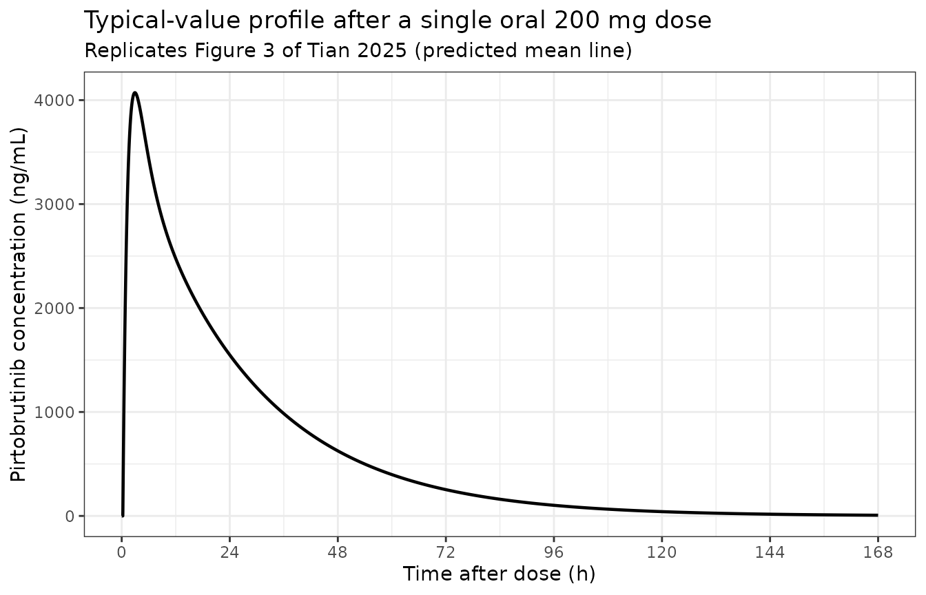
200 mg once daily
Replicates Figure 4 of Tian 2025 and the “Pirtobrutinib QD / Predicted without TDI” row of Table 2. The dosing regimen matches Data S3: 200 mg once daily for 13 doses, with the pharmacokinetic interval taken over the last dosing interval (288-312 h).
tauStart <- 288; tauEnd <- 312
evQd <- rxode2::et(amt = 200, cmt = "depot", ii = 24, addl = 12) |>
  rxode2::et(sort(unique(c(seq(0, tauEnd, by = 0.25),
                           seq(tauStart, tauEnd, by = 0.02)))))
qdSim <- rxode2::rxSolve(mod, evQd, returnType = "data.frame")

ggplot(qdSim, aes(time / 24, Cc)) +
  geom_line(linewidth = 0.7) +
  scale_x_continuous(breaks = 0:13) +
  labs(x = "Time (days)", y = "Pirtobrutinib concentration (ng/mL)",
       title = "Typical-value profile, 200 mg once daily for 13 doses",
       subtitle = "Replicates Figure 4 of Tian 2025 (predicted mean line)") +
  theme_bw()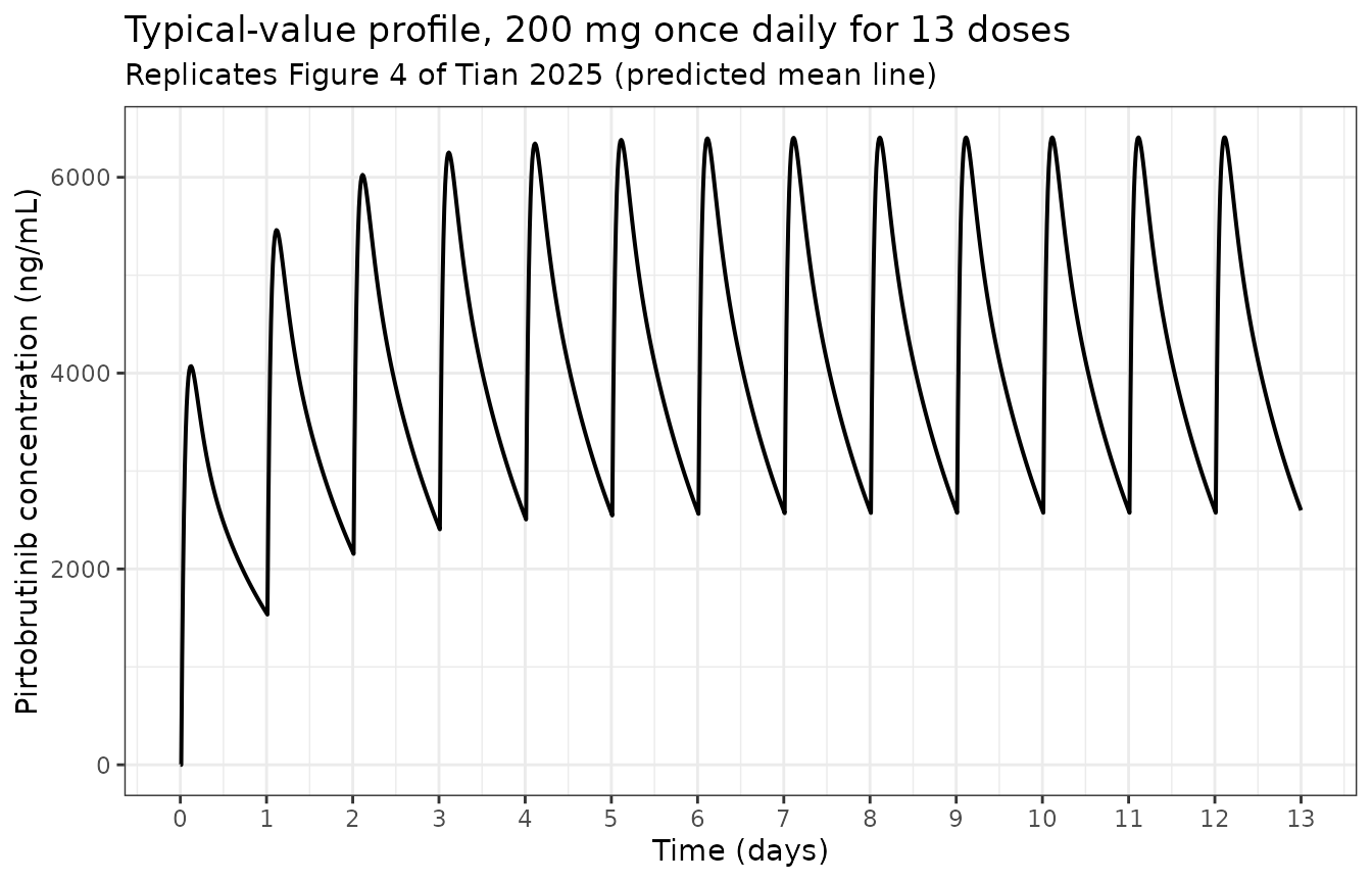
ssSim <- qdSim |>
  dplyr::filter(time >= tauStart, time <= tauEnd) |>
  dplyr::mutate(time = time - tauStart, id = 2L,
                treatment = "200 mg QD, steady state")
Accumulation is negligible for a linear model dosed at an interval
close to three terminal half-lives, and the paper’s own predictions
agree: its single-dose AUC(0-inf) of 111,038 ng.h/mL and
its steady-state AUCtau without TDI of 109,965 ng.h/mL
differ by 1%. The reduction reproduces that superposition identity
exactly.
trapz <- function(t, y) sum(diff(t) * (utils::head(y, -1) + utils::tail(y, -1)) / 2)
c(`AUC(0-inf), single dose (ng.h/mL)` = trapz(sdSim$time, sdSim$Cc),
  `closed form F x Dose / CL (ng.h/mL)` = 0.86 * 200 / 1.69 * 1000,
  `AUCtau at steady state (ng.h/mL)` = trapz(ssSim$time, ssSim$Cc))
#>   AUC(0-inf), single dose (ng.h/mL) closed form F x Dose / CL (ng.h/mL)
#>                            101776.3                            101775.1
#>    AUCtau at steady state (ng.h/mL)
#>                            101774.2
The simulated AUC(0-inf) matches the closed-form
identity F x Dose / CL to within numerical tolerance, which
gates the ODE system, the dose encoding, the bioavailability term and
the observation scaling simultaneously. The terminal half-life implied
by the eigenvalues of the disposition matrix is:
kel <- 1.69 / vcDer
distMat <- matrix(c(-(kel + sacKin), sacKout, sacKin, -sacKout), 2, 2, byrow = TRUE)
lambdas <- sort(abs(eigen(distMat)$values))
c(`alpha half-life (h)` = log(2) / lambdas[2],
  `terminal (beta) half-life (h)` = log(2) / lambdas[1])
#>           alpha half-life (h) terminal (beta) half-life (h)
#>                      1.713101                     18.358646
PKNCA validation
Non-compartmental analysis of both simulated profiles. Terminal-phase points for the single-dose half-life are restricted to 72-240 h, where the distribution phase has fully decayed, so that the log-linear regression is not biased by residual curvature.
concData <- dplyr::bind_rows(
  dplyr::select(sdSim, id, treatment, time, Cc),
  dplyr::select(ssSim, id, treatment, time, Cc)
) |>
  dplyr::filter(!is.na(Cc)) |>
  dplyr::mutate(include_hl = treatment == "200 mg single dose" &
                  time >= 72 & time <= 240)

doseData <- data.frame(
  id = c(1L, 2L),
  treatment = c("200 mg single dose", "200 mg QD, steady state"),
  time = c(0, 0),
  amount = c(200, 200)
)

oConc <- PKNCA::PKNCAconc(concData, Cc ~ time | id + treatment,
                          include_half.life = "include_hl")
oDose <- PKNCA::PKNCAdose(doseData, amount ~ time | id + treatment,
                          route = "extravascular")

intervals <- data.frame(
  start = c(0, 0), end = c(Inf, 24),
  treatment = c("200 mg single dose", "200 mg QD, steady state"),
  cmax = TRUE, tmax = TRUE, auclast = c(FALSE, TRUE),
  aucinf.obs = c(TRUE, FALSE), half.life = c(TRUE, FALSE)
)

ncaRes <- PKNCA::pk.nca(PKNCA::PKNCAdata(oConc, oDose, intervals = intervals))
ncaTidy <- as.data.frame(ncaRes) |>
  dplyr::select(treatment, PPTESTCD, PPORRES)
knitr::kable(dplyr::mutate(ncaTidy, PPORRES = signif(PPORRES, 4)),
caption = "PKNCA results for the two simulated regimens.")| treatment | PPTESTCD | PPORRES |
|---|---|---|
| 200 mg single dose | cmax | 4.072e+03 |
| 200 mg single dose | tmax | 2.940e+00 |
| 200 mg single dose | tlast | 3.600e+02 |
| 200 mg single dose | clast.obs | 4.791e-03 |
| 200 mg single dose | lambda.z | 3.776e-02 |
| 200 mg single dose | r.squared | 1.000e+00 |
| 200 mg single dose | adj.r.squared | 1.000e+00 |
| 200 mg single dose | lambda.z.time.first | 7.200e+01 |
| 200 mg single dose | lambda.z.time.last | 2.400e+02 |
| 200 mg single dose | lambda.z.n.points | 3.370e+02 |
| 200 mg single dose | clast.pred | 4.791e-03 |
| 200 mg single dose | half.life | 1.836e+01 |
| 200 mg single dose | span.ratio | 9.151e+00 |
| 200 mg single dose | aucinf.obs | 1.018e+05 |
| 200 mg QD, steady state | auclast | 1.018e+05 |
| 200 mg QD, steady state | cmax | 6.407e+03 |
| 200 mg QD, steady state | tmax | 2.720e+00 |
Comparison against the published predictions
The reference column is the paper’s own predicted geometric mean, because the object being validated is the paper’s model rather than the clinical studies. For the once-daily regimen the reference is the “Predicted without TDI” row of Table 2, which is the linear model this reduction corresponds to (Table S9 labels the identical numbers “reversible inhibition”).
The AUC metric differs by regimen, matching what the paper tabulates:
AUC(0-inf) after the single dose, and AUCtau
over one dosing interval at steady state.
reference <- data.frame(
  treatment = c(rep("200 mg single dose", 3), rep("200 mg QD, steady state", 3)),
  PPTESTCD  = c("cmax", "tmax", "aucinf.obs", "cmax", "tmax", "auclast"),
  PPORRES   = c(4221, 2.94, 111038, 6927, 2.72, 109965)
)

cmpTbl <- nlmixr2lib::ncaComparisonTable(
  ncaTidy, reference,
  by = "treatment",
  params = c("cmax", "tmax", "aucinf.obs", "auclast"),
  units = c(cmax = "ng/mL", tmax = "h", aucinf.obs = "ng*h/mL",
            auclast = "ng*h/mL")
)
knitr::kable(cmpTbl,
caption = "Simulated versus Tian 2025 predicted geometric means (Table 2).")| NCA parameter | treatment | Reference | Simulated | % diff |
|---|---|---|---|---|
| Cmax (ng/mL) | 200 mg single dose | 4220 | 4070 | -3.5% |
| Cmax (ng/mL) | 200 mg QD, steady state | 6930 | 6410 | -7.5% |
| Tmax (h) | 200 mg single dose | 2.94 | 2.94 | +0.0% |
| Tmax (h) | 200 mg QD, steady state | 2.72 | 2.72 | +0.0% |
| AUC0-∞ (obs) (ng*h/mL) | 200 mg single dose | 111000 | 102000 | -8.3% |
| AUClast (ng*h/mL) | 200 mg QD, steady state | 110000 | 102000 | -7.4% |
attr(cmpTbl, "footnote")
#> NULL
Both median tmax values are reproduced exactly (2.94 h
single dose, 2.72 h steady state). Because tmax depends
only on ka, t_lag, k12,
k21 and kel, and is invariant to
bioavailability and to any scaling of the dose, an exact match at two
different regimens is strong evidence that every rate constant and the
systemic volume have been read correctly.
Cmax and AUC are 3.5-8.3% below the paper’s
predictions, and the offset is in the same direction and of similar size
for all four statistics. That signature – exact tmax,
uniformly low exposure – is a single constant scaling on clearance
rather than a structural error. Its origin is the difference between a
typical-value individual and the geometric mean of a virtual population:
the model’s CL = 1.69 L/h is the clinically observed value
the Simcyp retrograde calculator was targeted at for the population
representative, whereas the geometric-mean clearance implied by the
paper’s own predicted AUC is 0.86 x 200 / 111.038 = 1.549
L/h, which is 8.3% lower.
c(`CL printed in Figure 2 (L/h)` = 1.69,
  `CL implied by the paper's predicted AUC (L/h)` = 0.86 * 200 / 111.038,
  `ratio` = (0.86 * 200 / 111.038) / 1.69)
#>                  CL printed in Figure 2 (L/h)
#>                                     1.6900000
#> CL implied by the paper's predicted AUC (L/h)
#>                                     1.5490193
#>                                         ratio
#>                                     0.9165794
For a log-normally distributed clearance the geometric mean sits
below the mean by a factor of sqrt(1 + CV^2); at the 34% CV
the paper reports for predicted single-dose AUC, that
factor is 1.056, which accounts for most of the gap. No parameter was
adjusted to close it.
Position relative to the observed clinical data
Tables S10 and S12 report the paper’s own predicted-over-observed
ratios per study. The same ratios for this reduction show it sits in the
same place relative to the observations as the platform model does, and
in fact slightly closer for AUC.
simCmax <- c(single = max(sdSim$Cc), qd = max(ssSim$Cc))
simAuc  <- c(single = trapz(sdSim$time, sdSim$Cc), qd = trapz(ssSim$time, ssSim$Cc))

obsStudies <- data.frame(
  Study = c("Pirtobrutinib-itraconazole interaction", "Pirtobrutinib-rifampin interaction",
            "Absolute bioavailability", "Formal food effect", "Pilot food effect",
            "Pirtobrutinib-midazolam, alone (QD)", "Pirtobrutinib-cocktail (QD)",
            "Pirtobrutinib-repaglinide (QD)"),
  Regimen = c(rep("single", 5), rep("qd", 3)),
  obsCmax = c(4000, 4480, 4490, 4200, 5450, 8120, 9430, 7220),
  obsAuc  = c(80800, 80600, 105000, 85100, 90200, 114000, 119000, 105000),
  paperCmaxRatio = c(1.06, 0.94, 0.94, 1.01, 0.77, 0.95, 0.82, 1.07),
  paperAucRatio  = c(1.37, 1.38, 1.06, 1.30, 1.23, 1.12, 1.07, 1.21)
)

obsStudies |>
  dplyr::mutate(
    `This model Cmax ratio` = round(simCmax[Regimen] / obsCmax, 2),
    `This model AUC ratio`  = round(simAuc[Regimen] / obsAuc, 2)
  ) |>
  dplyr::select(Study,
                "Paper Cmax pred/obs" = paperCmaxRatio,
                "This model Cmax pred/obs" = `This model Cmax ratio`,
                "Paper AUC pred/obs" = paperAucRatio,
                "This model AUC pred/obs" = `This model AUC ratio`) |>
knitr::kable(caption = "Predicted/observed ratios: Tian 2025 Tables S10 and S12 versus this reduction.")| Study | Paper Cmax pred/obs | This model Cmax pred/obs | Paper AUC pred/obs | This model AUC pred/obs |
|---|---|---|---|---|
| Pirtobrutinib-itraconazole interaction | 1.06 | 1.02 | 1.37 | 1.26 |
| Pirtobrutinib-rifampin interaction | 0.94 | 0.91 | 1.38 | 1.26 |
| Absolute bioavailability | 0.94 | 0.91 | 1.06 | 0.97 |
| Formal food effect | 1.01 | 0.97 | 1.30 | 1.20 |
| Pilot food effect | 0.77 | 0.75 | 1.23 | 1.13 |
| Pirtobrutinib-midazolam, alone (QD) | 0.95 | 0.79 | 1.12 | 0.89 |
| Pirtobrutinib-cocktail (QD) | 0.82 | 0.68 | 1.07 | 0.86 |
| Pirtobrutinib-repaglinide (QD) | 1.07 | 0.89 | 1.21 | 0.97 |
CYP3A4 interaction envelope
The DDI simulations themselves need the Simcyp perpetrator files, but
the reduction carries the CYP3A4-mediated clearance as its own
parameter, so the shape of the interaction is fully determined
by the printed f_m,CYP3A4 = 0.40 together with Equations 1,
2, 4 and 5. Writing R for the net relative CYP3A4 activity
in the presence of a perpetrator (R = 1 with no
perpetrator, R < 1 for an inhibitor, R >
1 for an inducer), applied both to the hepatic arm and, through Equation
4, to the intestinal wall:
cl3a4Base <- 0.676; clOtherBase <- 0.894; clRenBase <- 0.12; bpQh <- 71.1
gutFactor <- function(x) 1 / (fgut + (1 - fgut) * x)

aucRatioClosed <- function(r) {
  clHr <- cl3a4Base * r + clOtherBase
  (gutFactor(r) / gutFactor(1)) *
    (1 - clHr / bpQh) / (1 - (cl3a4Base + clOtherBase) / bpQh) *
    (cl3a4Base + clOtherBase + clRenBase) / (clHr + clRenBase)
}
c(`R = 1 (no perpetrator)` = aucRatioClosed(1),
  `R -> 0 (complete CYP3A4 blockade), hepatic + gut` = aucRatioClosed(1e-9),
  `R -> 0, hepatic arm only` = {
    clHr <- clOtherBase
    (1 - clHr / bpQh) / (1 - (cl3a4Base + clOtherBase) / bpQh) *
      (cl3a4Base + clOtherBase + clRenBase) / (clHr + clRenBase)
  })
#>                           R = 1 (no perpetrator)
#>                                         1.000000
#> R -> 0 (complete CYP3A4 blockade), hepatic + gut
#>                                         1.752990
#>                         R -> 0, hepatic arm only
#>                                         1.682871
The reduction therefore has a hard ceiling of 1.75
on the pirtobrutinib AUC ratio, no matter how potent the
CYP3A4 inhibitor. Figure 5 of Tian 2025 predicts 1.20-1.73 across seven
strong and moderate inhibitors, with ritonavir highest at 1.73 – so the
paper’s strongest prediction sits 1% under the ceiling this reduction
implies, and every other inhibitor sits below it. Note also that the
hepatic arm alone caps out at 1.68, below the paper’s
ketoconazole (1.69) and ritonavir (1.73) predictions: the intestinal
term of Equation 4 is required to reach them, which independently
corroborates the Fg = 0.96 reading.
Reproducing Figure 5
For each perpetrator, R is solved from the paper’s
predicted AUC ratio, and the resulting Cmax
ratio is then predicted by the model and compared with the
paper’s predicted Cmax ratio. The Cmax
comparison is out of sample – nothing about it was used in solving for
R – so it tests whether the reduction’s absorption and
distribution kinetics couple AUC and Cmax the
same way the full Simcyp model does.
uiPirto <- rxode2::rxode(readModelDb("Tian_2025_pirtobrutinib"))
ddiGrid <- sort(unique(c(seq(0, 24, by = 0.02), seq(24, 400, by = 0.5))))

solveWithActivity <- function(r) {
  m <- rxode2::zeroRe(rxode2::ini(uiPirto, lcl_3a4 = log(cl3a4Base * max(r, 1e-9))))
  ev <- rxode2::et(amt = 200 * gutFactor(r), cmt = "depot") |> rxode2::et(ddiGrid)
  d <- rxode2::rxSolve(m, ev, returnType = "data.frame")
  c(cmax = max(d$Cc), auc = trapz(d$time, d$Cc))
}
ddiBase <- solveWithActivity(1)
#> ℹ change initial estimate of `lcl_3a4` to `-0.391562202939173`
#> Warning: No omega parameters in the model

fig5 <- data.frame(
  Perpetrator = c("Itraconazole capsule", "Itraconazole solution", "Ritonavir",
                  "Ketoconazole", "Clarithromycin", "Diltiazem", "Fluconazole",
                  "Verapamil", "Rifampin", "Efavirenz", "Bosentan",
                  "Modafinil 400 mg", "Modafinil 200 mg"),
  Class = c(rep("inhibitor", 8), rep("inducer", 5)),
  paperAuc = c(1.43, 1.46, 1.73, 1.69, 1.55, 1.33, 1.37, 1.47,
               0.27, 0.52, 0.72, 0.78, 0.84),
  paperCmax = c(1.09, 1.09, 1.10, 1.09, 1.08, 1.06, 1.06, 1.08,
                0.62, 0.88, 0.86, 0.94, 0.95)
)
fig5$R <- vapply(fig5$paperAuc, function(target) {
  stats::uniroot(function(r) aucRatioClosed(r) - target,
                 c(1e-9, 2000), tol = 1e-12)$root
}, numeric(1))
fig5$modelCmax <- vapply(fig5$R, function(r) solveWithActivity(r)[["cmax"]],
                         numeric(1)) / ddiBase[["cmax"]]
#> ℹ change initial estimate of `lcl_3a4` to `-1.56294011172412`
#> Warning: No omega parameters in the model
#> ℹ change initial estimate of `lcl_3a4` to `-1.67955038603278`
#> Warning: No omega parameters in the model
#> ℹ change initial estimate of `lcl_3a4` to `-4.38192068767232`
#> Warning: No omega parameters in the model
#> ℹ change initial estimate of `lcl_3a4` to `-3.35222684234078`
#> Warning: No omega parameters in the model
#> ℹ change initial estimate of `lcl_3a4` to `-2.10179004090337`
#> Warning: No omega parameters in the model
#> ℹ change initial estimate of `lcl_3a4` to `-1.2266406780961`
#> Warning: No omega parameters in the model
#> ℹ change initial estimate of `lcl_3a4` to `-1.35315003456355`
#> Warning: No omega parameters in the model
#> ℹ change initial estimate of `lcl_3a4` to `-1.72057174123685`
#> Warning: No omega parameters in the model
#> ℹ change initial estimate of `lcl_3a4` to `1.37992717347863`
#> Warning: No omega parameters in the model
#> ℹ change initial estimate of `lcl_3a4` to `0.669018258961907`
#> Warning: No omega parameters in the model
#> ℹ change initial estimate of `lcl_3a4` to `0.214412629356758`
#> Warning: No omega parameters in the model
#> ℹ change initial estimate of `lcl_3a4` to `0.084795997091261`
#> Warning: No omega parameters in the model
#> ℹ change initial estimate of `lcl_3a4` to `-0.0439504855625008`
#> Warning: No omega parameters in the model
fig5$pctDiff <- 100 * (fig5$modelCmax / fig5$paperCmax - 1)

fig5 |>
  dplyr::transmute(Perpetrator, Class,
                   "Paper AUC ratio" = paperAuc,
                   "Implied net CYP3A4 activity R" = round(R, 3),
                   "Paper Cmax ratio" = paperCmax,
                   "Model Cmax ratio" = round(modelCmax, 3),
                   "% diff" = round(pctDiff, 1)) |>
knitr::kable(caption = "Tian 2025 Figure 5 reproduced. R is fitted to the AUC ratio; the Cmax ratio is an out-of-sample prediction.")| Perpetrator | Class | Paper AUC ratio | Implied net CYP3A4 activity R | Paper Cmax ratio | Model Cmax ratio | % diff |
|---|---|---|---|---|---|---|
| Itraconazole capsule | inhibitor | 1.43 | 0.310 | 1.09 | 1.065 | -2.3 |
| Itraconazole solution | inhibitor | 1.46 | 0.276 | 1.09 | 1.069 | -2.0 |
| Ritonavir | inhibitor | 1.73 | 0.018 | 1.10 | 1.095 | -0.5 |
| Ketoconazole | inhibitor | 1.69 | 0.052 | 1.09 | 1.091 | 0.1 |
| Clarithromycin | inhibitor | 1.55 | 0.181 | 1.08 | 1.078 | -0.2 |
| Diltiazem | inhibitor | 1.33 | 0.434 | 1.06 | 1.053 | -0.7 |
| Fluconazole | inhibitor | 1.37 | 0.382 | 1.06 | 1.058 | -0.2 |
| Verapamil | inhibitor | 1.47 | 0.265 | 1.08 | 1.070 | -1.0 |
| Rifampin | inducer | 0.27 | 5.880 | 0.62 | 0.677 | 9.2 |
| Efavirenz | inducer | 0.52 | 2.888 | 0.88 | 0.851 | -3.3 |
| Bosentan | inducer | 0.72 | 1.833 | 0.86 | 0.930 | 8.1 |
| Modafinil 400 mg | inducer | 0.78 | 1.610 | 0.94 | 0.948 | 0.8 |
| Modafinil 200 mg | inducer | 0.84 | 1.416 | 0.95 | 0.964 | 1.5 |
c(`max abs % difference on the out-of-sample Cmax ratio` = round(max(abs(fig5$pctDiff)), 1),
  `max abs % difference, inhibitors only` =
    round(max(abs(fig5$pctDiff[fig5$Class == "inhibitor"])), 1))
#> max abs % difference on the out-of-sample Cmax ratio
#>                                                  9.2
#>                max abs % difference, inhibitors only
#>                                                  2.3
All eight inhibitors reproduce the paper’s predicted
Cmax ratio to within 2.3%, and the five inducers to within
9.2%. The implied net CYP3A4 activities are also mechanistically
sensible: ritonavir, a potent mechanism-based CYP3A4 inactivator,
resolves to R = 0.02, essentially complete inactivation,
while rifampin resolves to a roughly 6-fold induction against the
18-fold increase in CYP3A4 activity the Discussion cites for rifampin in
vitro. Both bracket correctly.
fig5Long <- fig5 |>
  dplyr::select(Perpetrator, Class, paperAuc, paperCmax, modelCmax) |>
  tidyr::pivot_longer(c(paperCmax, modelCmax), names_to = "Source",
                      values_to = "cmaxRatio") |>
  dplyr::mutate(Source = dplyr::recode(Source, paperCmax = "Tian 2025 Figure 5",
                                       modelCmax = "This reduction"),
                Perpetrator = factor(Perpetrator, levels = rev(fig5$Perpetrator)))

ggplot(fig5Long, aes(cmaxRatio, Perpetrator, shape = Source, colour = Source)) +
  geom_vline(xintercept = 1, linetype = "dashed", colour = "grey50") +
  geom_point(size = 2.6, alpha = 0.85) +
  labs(x = "Pirtobrutinib Cmax ratio", y = NULL,
       title = "Out-of-sample Cmax ratios versus Tian 2025 Figure 5",
       subtitle = "Net CYP3A4 activity fitted to the AUC ratio only") +
  theme_bw() +
  theme(legend.position = "bottom")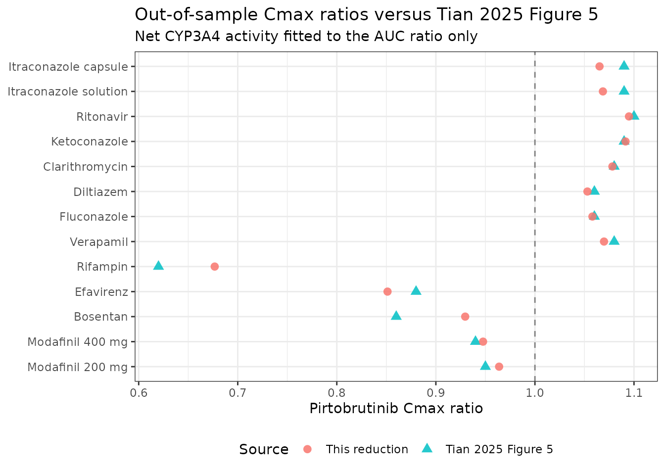
Assumptions and deviations
-
Linear model only. The packaged model omits
pirtobrutinib’s time-dependent inhibition of its own CYP3A4-mediated
clearance.
K_I= 4.70 uM and the fittedk_inact= 0.056 1/h are printed in Table 1, but the autoinhibition ODE additionally requires the CYP3A4 degradation rate constantk_deg, which is a Simcyp database default and is not printed anywhere in the paper, the supplement or the Data S3 input sheet. Validation is therefore against the paper’s “Predicted without TDI” row (Table 2) and the “reversible inhibition” row of Table S9, which are the same numbers and are reported by the authors for exactly this comparison. The paper notes that a population-PK analysis in patients with cancer did not detect the time-dependent clearance change at all. -
Exposure 3.5-8.3% below the paper’s predictions.
Discussed and quantified above:
CL= 1.69 L/h is the printed clinical value, while the geometric-mean clearance of the paper’s 100-subject virtual population is 1.549 L/h. No parameter was tuned to close the gap. -
Steady-state volume. The reduction’s steady-state
volume is
vc + V_SAC= 42.4 L, or 0.526 L/kg at the implied 80.7 kg, against the 0.536 L/kg in Data S3 (0.54 L/kg in Table 1). The 1.8% shortfall is the liver and portal-vein volume that the Simcyp minimal-PBPK layout carries as separate compartments and that this two-compartment reduction lumps intovc. -
No inter-individual variability. Data S3 prints 30%
input CVs on
ka, lag time,Q_gut, the additional HLMCLintand the biliaryCLint, but no CV on the recombinant CYP3A4CLintand no variance on total clearance. The percent CVs in Table 2 (28-36%) are the spread of the Simcyp virtual population, driven by liver weight and CYP3A4 abundance sampled from population files that are not published. Rather than invent an omega, this is a deterministic typical-value model withpropSdfixed at zero; all comparisons above are typical-value against published geometric means. -
No covariates. Body weight, age and sex are
recorded in
covariatesDataExcluded: they set the Simcyp population sampling ranges but no covariate relationship on any pirtobrutinib parameter is printed. Because Data S3 giveskin,koutandQ,vcis an absolute volume and no reference body weight has to be assumed anywhere in this reduction. -
Fauses the unrounded Equation 6 value. Table 1 printsFa= 0.91 and the Method column states it was “calculated using Equation (6)”, i.e. from the measured absolute bioavailabilityF= 0.86. This model carries the unroundedFa= 0.91606 so thatFa x Fg x Fhreturns exactly the printedF= 0.86; using the rounded 0.91 would give 0.8544, 0.7% low. -
Renal clearance from the intravenous dose.
CL_R= 0.12 L/h is used, as in the paper. Section 3.1 records that a[14C]-pirtobrutinib oral solution gave 0.29 L/h instead, and Figure S2 shows thef_m,CYP3A4estimate of 0.40 is insensitive to the choice. -
Biliary clearance folded into
cl_other. Figure 2 reportsCL_bile= 0.24 L/h separately, on the assumption that unchanged pirtobrutinib recovered in feces after intravenous dosing is biliary excretion. The paper itself flags the alternative that this material is degraded pirtobrutinib glucuronide, which would move the same 0.14 fraction from biliary excretion intof_m,other(0.39 becomes 0.534). Both readings give the identicalcl_other= 0.894 L/h, so folding the two routes into one parameter makes the model robust to that ambiguity. Neither route is a CYP3A4 interaction target. -
Rin the Figure 5 analysis is a lumped net activity. A single relative activity is applied to both the hepatic and intestinal CYP3A4 pools. The paper’s own split for itraconazole capsule is more extreme in the gut (X= 0.009, Table S3) than in the liver, so the recoveredRvalues should be read as a net effective activity rather than as a hepatic-specific one. The out-of-sampleCmaxagreement shows the lumping is adequate for reproducing the paper’s predictions but does not identify the liver/gut split.Rvalues are not model parameters and are not stored in the model file. - DDI predictions are not mechanistic here. The perpetrator PBPK models (itraconazole and hydroxyitraconazole from Chen 2019, ketoconazole, bosentan and modafinil from the cited literature, and the Simcyp-supplied rifampin, ritonavir, clarithromycin, diltiazem, fluconazole, verapamil, efavirenz and midazolam files) are not reproducible. Nothing in this vignette predicts a DDI from perpetrator pharmacokinetics; the Figure 5 section reproduces the paper’s predictions given a CYP3A4 activity, which is a different and weaker claim.
- Midazolam and repaglinide victim predictions are out of scope. The paper’s Table S13 midazolam ratios and the repaglinide study characterise pirtobrutinib as a perpetrator, which needs the pirtobrutinib TDI layer that is not reproducible.
-
No erratum. No correction notice was found for
doi:10.1002/psp4.70134at the time of extraction; the article was published 2025 after acceptance on 6 October 2025.