Anti-CD66 radioimmunotherapy whole-body PBPK (Kletting 2015)

Model and source

• Citation: Kletting P, Maass C, Reske S, Beer AJ, Glatting G. Physiologically Based Pharmacokinetic Modeling Is Essential in 90Y-Labeled Anti-CD66 Radioimmunotherapy. PLoS One. 2015;10(5):e0127934. doi:10.1371/journal.pone.0127934. Model equations, fixed parameters and data-assignment equations are in supplement S1 Text (Eqs 1-43, Tables A and B); per-patient administered amounts and fitting results are in supplement S1 Table.
• Article: https://doi.org/10.1371/journal.pone.0127934
• S1 Text (model equations and parameters): https://doi.org/10.1371/journal.pone.0127934.s004
• S1 Table (per-patient data and fitting results): https://doi.org/10.1371/journal.pone.0127934.s003
• ODE states per model: 86

Radioimmunotherapy with the murine anti-CD66 antibody BW 250/183 is used to intensify conditioning before stem-cell transplantation in acute leukaemia. The dose the red marrow receives is computed from a time-integrated activity coefficient, the area under the organ’s time-activity curve divided by the injected activity, and that coefficient has to be predicted from a small pre-therapeutic tracer administration of 111In-labelled antibody before the much larger therapeutic administration of 90Y-labelled antibody is given.

Kletting and co-workers show that this prediction fails if the tracer and the therapy are assumed to behave alike. The number of CD66 antigens available in the red marrow – about 20 nmol – is the same order of magnitude as the amount of antibody given for therapy – about 9 nmol – so the therapeutic administration partially saturates the marrow and a larger fraction of it stays in serum. Assuming equal biodistributions underestimates the serum coefficient by (-25 +/- 16)%. Their refined PBPK model predicts the difference to (-3 +/- 20)%.

Two refinements produce that improvement, and both are in the model files here. The first is immunoreactivity. An antibody arm is immunoreactive with probability r_im, so the injected material splits into fully (r_im^2), half (2 r_im (1 - r_im)) and non-immunoreactive ((1 - r_im)^2) species with genuinely different binding: fully immunoreactive antibody can crosslink two antigens and is bound far more tightly than half immunoreactive antibody, which can only bind one. The fitted r_im is about 0.80, not 1, so roughly a third of the injected antibody is half immunoreactive and a further 4 % binds nothing at all. The second is a constraint on the red marrow antigen number, which is the parameter that matters most for dosimetry and is the one that cannot be measured: it is tied to the fitted liver and spleen antigen numbers through published granulocyte-pool ratios rather than estimated freely.

Each of the three immunoreactivity species is carried as a radiolabelled and an unlabelled copy – six parallel circulations – coupled only by physical decay, which converts a labelled molecule into an unlabelled one wherever it happens to be, and competing for one shared antigen pool. That is what makes the residual antibody from the tracer administration matter: by the time therapy is given it is mostly unlabelled, invisible to the camera, and still occupying antigen.

The paper fits two models that differ only in how the blood antigen number is constrained, and averages their predictions with Akaike weights of 0.51 +/- 0.17 and 0.49 +/- 0.17. Both are shipped: Kletting_2015_antiCD66_pbpk_model1 uses the unweighted liver-plus-spleen sum (S1 Text Eq 8) and Kletting_2015_antiCD66_pbpk_model2 weights each organ by its measured over calculated volume (S1 Text Eq 9), to compensate for the hepatomegaly and splenomegaly common in acute leukaemia.

Population

str(readModelDb("Kletting_2015_antiCD66_pbpk_model1")()$population)
#> List of 7
#>  $ species      : chr "human"
#>  $ n_subjects   : num 27
#>  $ n_studies    : num 2
#>  $ disease_state: chr "acute leukaemia (21 acute myeloid, 6 acute lymphoblastic); radioimmunotherapy to intensify conditioning before "| __truncated__
#>  $ dose_range   : chr "Pre-therapeutic imaging: 0.5 +/- 0.1 mg anti-CD66 antibody (1 mg = 6.7 nmol; 3.3 +/- 0.6 nmol in S1 Table) carr"| __truncated__
#>  $ regions      : chr "Germany (Ulm University)"
#>  $ notes        : chr "Both study protocols were approved by the Ethics Committee of Ulm University. Age, sex, weight and height distr"| __truncated__

Twenty-seven patients with acute leukaemia (21 acute myeloid, 6 acute lymphoblastic) were studied under two protocols at Ulm University. Each patient was fitted individually – 27 separate SAAM II fits, not a population model – so Table 1 reports the mean and SD of 27 individual estimates rather than a typical value and an omega. The model files ship those means as the typical values and record the SDs in population$notes; they are estimation-error inflated individual spreads and are deliberately not encoded as inter-individual variability. The paper reports no age, sex, weight or height distribution, so this vignette uses a 70 kg, 170 cm reference adult.

Source trace

Every value in either ini() block, and every equation in model(), with its location in the source. S1 Text is the supplement (journal.pone.0127934.s004).

Quantity	Source	Value
Ag0,L, Ag0,S – liver and spleen antigen numbers	Table 1	0.31 / 0.22 nmol (model 1); 0.33 / 0.25 (model 2)
exL, exS – extravascular delay fractions	Table 1	0.235 / 0.107 (model 1); 0.226 / 0.098 (model 2)
fRM – fraction of plasma flow to red marrow	Table 1	0.67 % (model 1); 0.73 % (model 2)
cRM – L2-L4 scaling correction	Table 1	1.22 (model 1); 1.20 (model 2)
lambda_db – degradation of bound antibody	Table 1	6.8e-5 /min (both models)
r_im – immunoreactivity probability	Table 1	0.801 (model 1); 0.806 (model 2)
V – total serum volume	Table 1	2.99 L (model 1); 3.00 L (model 2)
k_on,mono, k_off	S1 Text Table B	0.006 L/nmol/min, 0.06 /min (fixed)
E – bivalent enhancement factor	S1 Text Table B	1 672 000 /cm
r_cell	S1 Text Table B	6.0 um
N_cells,RM	S1 Text Table B	188e8 per kg x BW
lambda_phy	S1 Text Table B	1.72e-4 /min (111In); 1.80e-4 /min (90Y)
k_in, k_out	S1 Text Table B	0.0017 /min, 0.005 /min
lambda_du, lambda_clex, lambda_cl	S1 Text Table B	3.9e-4, 3.9e-5, 0.047 /min
lambda_Metaex1..4	S1 Text Table B	0.39, 0.17, 0.018, 0.013 /min
V_RM, V_GI, V_L, V_S as fractions of V	S1 Text Eq 1	0.04, 0.076, 0.1, 0.014
F = 1.23 V; F_L, F_S, F_GI fractions	S1 Text Table B	0.065, 0.03, 0.16 of F
intL, intS; V_ROI,L2-L4	S1 Text Table A and B	0.04, 0.04; 30 mL
K = (170 / height) / 0.06665	S1 Text Table A	UlmDos scaling factor
a, b – radiochemical purities	S1 Text Table B	0.94 (tracer), 0.96 (therapy)
f_l,PT, f_l,T – labelled antibody fractions	S1 Text Table B	2.3 %, 21 %
Free antigen balance	S1 Text Eq 2	Ag_i = Ag0,i - mono - 2 x bi - ha mono
Bivalent enhancement alpha_i	S1 Text Eq 3	E / (4 pi r_cell^2 N_cells,i)
Ag0,RM = 38 Ag0,B	S1 Text Eq 4	granulocyte pool ratio, ref [7]
Blood antigen constraint	S1 Text Eqs 5-9	model 1 Eq 8; model 2 Eq 9
Injected amounts and r_im split	S1 Text Eqs 10-16	f() in model()
Liver / spleen / serum / red marrow readouts	S1 Text Eqs 17-21	abLiverRoi, abSpleenRoi, Cc, abMarrowRoi
Fully immunoreactive ODEs	S1 Text Eqs 22-28	agbi_fa_, agmono_fa_, ab_fa_*
Half immunoreactive ODEs	S1 Text Eqs 29-34	agmono_ha_, ab_ha_
Non-immunoreactive ODEs	S1 Text Eqs 35-39	ab_na_*
Degraded-antibody submodel	S1 Text Eqs 40-43	ex_, metap_, metaex1_, metaex2_
Administered antibody amounts	Methods 2.1 and S1 Table	3.25 nmol tracer, 8.75 nmol therapy (cohort means)

Virtual subject and dosing

The paper reports no demographics, so the subject is the 70 kg, 170 cm reference adult; WT enters only the cell numbers behind the bivalent enhancement factor and HT only the L2-L4 readout.

Administered amounts are the S1 Table cohort means: 3.25 nmol of antibody for the pre-therapeutic tracer and 8.75 nmol for therapy (1 mg = 6.7 nmol, so 0.49 mg and 1.31 mg, matching the 0.5 +/- 0.1 mg and 1.3 +/- 0.5 mg of Methods 2.1). The radiolabelled fraction is a x f_l,PT = 0.94 x 0.023 = 0.0216 for the tracer and b x f_l,T = 0.96 x 0.21 = 0.2016 for therapy.

That labelled fraction is checkable against the activities the paper reports, because one nmol of a nuclide carries a fixed activity lambda_phy x N_A:

NA_avo <- 6.02214076e23
specAct <- function(lambdaPerMin) lambdaPerMin / 60 * 1e-9 * NA_avo   # Bq per nmol
tibble::tibble(
  Nuclide = c("111In", "90Y"),
  `Labelled antibody (nmol)` = c(3.2517 * 0.0216, 8.7478 * 0.2016),
  `Implied activity (GBq)` = c(3.2517 * 0.0216 * specAct(1.72e-4),
                               8.7478 * 0.2016 * specAct(1.80e-4)) / 1e9,
  `Paper (Methods 2.1)` = c("0.130 +/- 0.016 GBq", "3.2 +/- 0.9 GBq")
) |>
  knitr::kable(digits = 3)

Nuclide	Labelled antibody (nmol)	Implied activity (GBq)	Paper (Methods 2.1)
111In	0.070	0.121	0.130 +/- 0.016 GBq
90Y	1.764	3.186	3.2 +/- 0.9 GBq

# The two labelled fractions are not free: they must reproduce the reported
# activities at carrier-free specific activity. Assert both to 15 %.
stopifnot(
  abs(3.2517 * 0.0216 * specAct(1.72e-4) / 1e9 / 0.130 - 1) < 0.15,
  abs(8.7478 * 0.2016 * specAct(1.80e-4) / 1e9 / 3.2 - 1) < 0.15
)

Dosing is six simultaneous bolus records into the six main vascular compartments, all carrying the same total antibody amount; the model’s f() block applies the labelled fraction and the r_im^2 : 2 r_im (1 - r_im) : (1 - r_im)^2 split (S1 Text Eqs 10-16), so the split lives in the model rather than in the event table.

doseCmt <- c("ab_fa_plasma_lab", "ab_ha_plasma_lab", "ab_na_plasma_lab",
             "ab_fa_plasma_unlab", "ab_ha_plasma_unlab", "ab_na_plasma_unlab")

#' Solve one administration.
#'
#' @param mod an rxode2 model
#' @param amt total antibody administered (nmol)
#' @param tmax end of the integration window (min)
#' @param inits optional named state vector to start from
solveOne <- function(mod, amt, tmax, inits = NULL) {
  ev <- rxode2::et(amt = amt, cmt = doseCmt[[1]], time = 0)
  for (cc in doseCmt[-1]) ev <- rxode2::et(ev, amt = amt, cmt = cc, time = 0)
  ev <- rxode2::et(ev, sort(unique(c(seq(0, 600, by = 2), seq(600, tmax, by = 20)))))
  dat <- as.data.frame(ev)
  dat$WT <- 70
  dat$HT <- 170
  args <- list(mod, dat, returnType = "data.frame", atol = 1e-10, rtol = 1e-8)
  if (!is.null(inits)) args$inits <- inits
  do.call(rxode2::rxSolve, args)
}

#' Trapezoidal time-integrated activity coefficient, in hours.
tiac <- function(s, col, labelledInjected) {
  y <- s[[col]]
  sum(diff(s$time) * (head(y, -1) + tail(y, -1)) / 2) / labelledInjected / 60
}

abPt <- 3.2517       # S1 Table: mean pre-therapeutic antibody (nmol)
abT <- 8.7478        # S1 Table: mean therapeutic antibody (nmol)
fracPt <- 0.0216     # a * f_l,PT
fracT <- 0.2016      # b * f_l,T
tmaxTiac <- 20000    # Methods 2.3: integration window for the coefficients

Simulation

Pre-therapeutic tracer administration

mod1 <- rxode2::rxode2(readModelDb("Kletting_2015_antiCD66_pbpk_model1"))
mod2 <- rxode2::rxode2(readModelDb("Kletting_2015_antiCD66_pbpk_model2"))

pre1 <- solveOne(mod1, abPt, tmaxTiac)
pre2 <- solveOne(mod2, abPt, tmaxTiac)
labPt <- abPt * fracPt

Replicates Figure 2 of Kletting 2015: the pre-therapeutic 111In time-activity curves for red marrow, liver, spleen and whole body, each as a percentage of the injected activity.

organs <- c(abWholeBody = "Whole body", abMarrow = "Red marrow",
            abLiverRoi = "Liver", abSpleenRoi = "Spleen")
pre1 |>
  dplyr::select(time, dplyr::all_of(names(organs))) |>
  tidyr::pivot_longer(-time, names_to = "state", values_to = "nmol") |>
  dplyr::mutate(Organ = factor(organs[state], levels = unname(organs)),
                pct = 100 * nmol / labPt) |>
  dplyr::filter(time > 0, time <= 8640) |>
  ggplot2::ggplot(ggplot2::aes(time / 60, pct, colour = Organ)) +
  ggplot2::geom_line(linewidth = 0.8) +
  ggplot2::scale_y_log10() +
  ggplot2::labs(x = "Time after the pre-therapeutic injection (h)",
                y = "Per cent of injected 111In activity", colour = NULL) +
  ggplot2::theme_bw()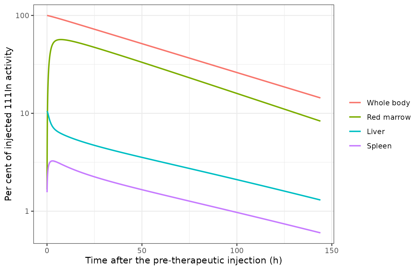

Replicates Figure 2A of Kletting 2015 (model 1, typical subject).

Therapy, with the tracer still on board

The therapeutic injection is given about eight days after the tracer (the first 90Y serum sample in S1 Table sits at 11527 min post-tracer for patient 1). Two things carry over: the antibody still in the body, and the saturation it causes. The tracer’s 111In label is irrelevant to a 90Y measurement, so the residual labelled states are folded into their unlabelled twins – the same antibody, still occupying antigen, no longer seen by the camera – and the therapy run starts from that state with lambda_phy switched to 90Y.

tTherapy <- 192 * 60

therapyFrom <- function(mod) {
  preAtT <- solveOne(mod, abPt, tTherapy)
  init <- unlist(preAtT[nrow(preAtT), mod$state])
  for (nm in grep("_lab$", mod$state, value = TRUE)) {
    unl <- sub("_lab$", "_unlab", nm)
    init[[unl]] <- init[[unl]] + init[[nm]]
    init[[nm]] <- 0
  }
  init
}

modT1 <- rxode2::rxode2(rxode2::ini(readModelDb("Kletting_2015_antiCD66_pbpk_model1"),
                                    lambdaPhy = 1.80e-4, fracLabeled = fracT))
#> ℹ change initial estimate of `lambdaPhy` to `0.00018`
#> ℹ change initial estimate of `fracLabeled` to `0.2016`
modT2 <- rxode2::rxode2(rxode2::ini(readModelDb("Kletting_2015_antiCD66_pbpk_model2"),
                                    lambdaPhy = 1.80e-4, fracLabeled = fracT))
#> ℹ change initial estimate of `lambdaPhy` to `0.00018`
#> ℹ change initial estimate of `fracLabeled` to `0.2016`

init1 <- therapyFrom(mod1)
init2 <- therapyFrom(mod2)
thr1 <- solveOne(modT1, abT, tmaxTiac, inits = init1)
thr2 <- solveOne(modT2, abT, tmaxTiac, inits = init2)
labT <- abT * fracT

residualAb <- sum(init1[grep("^(ab|agmono|agbi)_", names(init1))])
cat("Intact antibody still present when therapy is given: ",
    signif(residualAb, 3), " nmol = ", round(100 * residualAb / abPt, 1),
    " % of the tracer dose\n", sep = "")
#> Intact antibody still present when therapy is given: 1.12 nmol = 34.3 % of the tracer dose

dplyr::bind_rows(
  dplyr::transmute(pre1, time, Administration = "Pre-therapeutic (111In)",
                   pct = 100 * Cc / labPt),
  dplyr::transmute(thr1, time, Administration = "Therapeutic (90Y)",
                   pct = 100 * Cc / labT)
) |>
  dplyr::filter(time > 0, time <= 8640) |>
  ggplot2::ggplot(ggplot2::aes(time / 60, pct, colour = Administration)) +
  ggplot2::geom_line(linewidth = 0.8) +
  ggplot2::scale_y_log10() +
  ggplot2::labs(x = "Time after injection (h)",
                y = "Per cent of injected activity per litre of serum",
                colour = NULL) +
  ggplot2::theme_bw()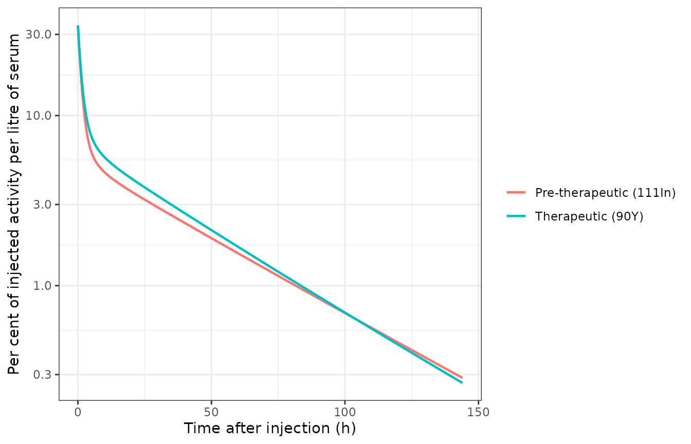

Replicates Figure 2B of Kletting 2015: serum time-activity curves, each normalised to its own injected activity.

Normalised to its own injected activity, the therapeutic curve carries the larger area: the bigger antibody amount saturates the marrow antigen, so proportionally more of the injected activity stays in serum. That is the paper’s central mechanism, and it is why the coefficients cannot simply be carried over.

Validation

1. Mass balance

The only route out of the system is lambda_cl from the plasma degradation product, so total antibody-derived mass must be conserved exactly.

massDev <- c(max(abs(pre1$abMassBalance / abPt - 1)),
             max(abs(pre2$abMassBalance / abPt - 1)))
cat("largest relative mass-balance deviation:", signif(max(massDev), 3), "\n")
#> largest relative mass-balance deviation: 2.4e-14
stopifnot(max(massDev) < 1e-8)

This is a strong structural check on an 86-state system: every flow term, every decay coupling and every binding term appears once as a gain and once as a loss, so a single mis-routed or mis-signed term breaks it.

2. The whole-body coefficient cannot exceed the physical mean life

With no excretion at all, the whole-body time-integrated activity coefficient would equal the mean life of the nuclide, 1 / lambda_phy.

meanLife <- 1 / 1.72e-4 / 60
wb <- tiac(pre1, "abWholeBody", labPt)
cat("whole-body coefficient", round(wb, 1), "h against the",
    round(meanLife, 1), "h physical bound\n")
#> whole-body coefficient 73.9 h against the 96.9 h physical bound
stopifnot(wb > 0, wb < meanLife)

3. Non-compartmental analysis of the serum curve

The serum coefficient the paper reports is a dose-normalised AUC, so PKNCA computes it directly. Cc is a concentration of labelled antibody in nmol/L, and the coefficient is the AUC over the paper’s 0 to 20 000 min window divided by the injected labelled amount.

ncaConc <- dplyr::bind_rows(
  dplyr::transmute(pre1, id = 1L, treatment = "Pre-therapeutic (111In)",
                   time, conc = Cc, dose = labPt),
  dplyr::transmute(thr1, id = 1L, treatment = "Therapeutic (90Y)",
                   time, conc = Cc, dose = labT)
) |>
  dplyr::filter(!is.na(conc))

ncaDose <- ncaConc |>
  dplyr::group_by(id, treatment) |>
  dplyr::summarise(dose = dplyr::first(dose), time = 0, .groups = "drop")

oConc <- PKNCA::PKNCAconc(as.data.frame(ncaConc), conc ~ time | id / treatment,
                          concu = "nmol/L", timeu = "min")
# PKNCAdose groups with `+`, not the nested `/` PKNCAconc accepts.
oDose <- PKNCA::PKNCAdose(as.data.frame(ncaDose), dose ~ time | id + treatment,
                          doseu = "nmol")
intervals <- data.frame(start = 0, end = tmaxTiac,
                        auclast = TRUE, cmax = TRUE, tmax = TRUE, half.life = TRUE)
res <- PKNCA::pk.nca(PKNCA::PKNCAdata(oConc, oDose, intervals = intervals))

ncaTab <- as.data.frame(res) |>
  dplyr::select(treatment, PPTESTCD, PPORRES) |>
  tidyr::pivot_wider(names_from = PPTESTCD, values_from = PPORRES)
ncaTab |>
  dplyr::mutate(`Coefficient a~serum (h/L)` = auclast / c(labPt, labT) / 60) |>
  dplyr::rename("Administration" = treatment, "AUClast (nmol/L*min)" = auclast,
                "Cmax (nmol/L)" = cmax, "Tmax (min)" = tmax,
                "Half-life (min)" = half.life) |>
  knitr::kable(digits = 4)

Administration	AUClast (nmol/L*min)	Cmax (nmol/L)	Tmax (min)	tlast	lambda.z	r.squared	adj.r.squared	lambda.z.time.first	lambda.z.time.last	lambda.z.n.points	clast.pred	Half-life (min)	span.ratio	Coefficient a~serum (h/L)
Pre-therapeutic (111In)	12.8172	0.0305	0	20000	3e-04	0.9999	0.9999	3700	20000	816	0e+00	2133.412	7.6403	3.0414
Therapeutic (90Y)	359.8264	0.7660	0	20000	3e-04	0.9999	0.9999	9200	20000	541	1e-04	2038.870	5.2971	3.4006

The PKNCA AUC and the trapezoidal integral used for the other organs must agree, which cross-checks the integration the rest of this vignette relies on. PKNCA’s default is linear-up / log-down and tiac() is a plain linear trapezoid, so they are not identical, but on this observation grid they must be within a per cent.

aucPre <- ncaTab$auclast[ncaTab$treatment == "Pre-therapeutic (111In)"]
cat("PKNCA / trapezoid ratio:",
    signif(aucPre / labPt / 60 / tiac(pre1, "Cc", labPt), 6), "\n")
#> PKNCA / trapezoid ratio: 0.999971
stopifnot(abs(aucPre / labPt / 60 / tiac(pre1, "Cc", labPt) - 1) < 0.01)

4. Table 2 – the published time-integrated activity coefficients

This is the end-to-end gate. Every organ coefficient in Table 2 has to fall out of the model at the Table 1 means, and the model-averaged prediction uses the paper’s Akaike weights of 0.51 and 0.49.

w1 <- 0.51; w2 <- 0.49
cols <- c(abMarrow = "Red marrow", abLiverRoi = "Liver", abSpleenRoi = "Spleen",
          Cc = "Serum [h/L]", abWholeBody = "Whole body")

tiacRow <- function(col) {
  c(m1 = tiac(pre1, col, labPt), m2 = tiac(pre2, col, labPt),
    t1 = tiac(thr1, col, labT), t2 = tiac(thr2, col, labT))
}
vals <- vapply(names(cols), tiacRow, numeric(4))

table2 <- tibble::tibble(
  Organ = unname(cols),
  `Pre-therapy, model averaged` = w1 * vals["m1", ] + w2 * vals["m2", ],
  `Paper pre-therapy` = c("42.2 +/- 7.7", "6.6 +/- 2.1", "3.1 +/- 1.3",
                          "3.8 +/- 1.4", "72.4 +/- 3.4"),
  `Therapy, model averaged` = w1 * vals["t1", ] + w2 * vals["t2", ],
  `Paper therapy` = c("37.3 +/- 7.5", "7.0 +/- 2.0", "2.9 +/- 0.9",
                      "4.9 +/- 1.8", "74.2 +/- 3.8")
)
knitr::kable(table2, digits = 2)

Organ	Pre-therapy, model averaged	Paper pre-therapy	Therapy, model averaged	Paper therapy
Red marrow	45.25	42.2 +/- 7.7	43.91	37.3 +/- 7.5
Liver	5.52	6.6 +/- 2.1	4.97	7.0 +/- 2.0
Spleen	2.58	3.1 +/- 1.3	2.13	2.9 +/- 0.9
Serum [h/L]	2.95	3.8 +/- 1.4	3.29	4.9 +/- 1.8
Whole body	73.75	72.4 +/- 3.4	71.92	74.2 +/- 3.8

paperPre <- c(42.2, 6.6, 3.1, 3.8, 72.4)
paperPreSd <- c(7.7, 2.1, 1.3, 1.4, 3.4)
modelPre <- table2$`Pre-therapy, model averaged`

# Every organ coefficient must land inside one between-patient SD of the
# published cohort mean. The comparison is a typical-parameter model against a
# mean of per-patient fits, so exact agreement is not expected; one SD is the
# right tolerance and is tight enough that a transcription error in any flow,
# volume, antigen number or binding constant fails it.
zScore <- abs(modelPre - paperPre) / paperPreSd
print(round(setNames(zScore, table2$Organ), 2))
#>  Red marrow       Liver      Spleen Serum [h/L]  Whole body 
#>        0.40        0.51        0.40        0.61        0.40
stopifnot(all(zScore < 1))

# The whole-body coefficient is the best determined of the five (the paper's own
# relative standard error is 1.1 %), so it gets a tighter bound.
stopifnot(abs(modelPre[5] / paperPre[5] - 1) < 0.05)

5. The mechanism: saturation raises the serum coefficient

The paper’s central quantitative claim is that the serum coefficient is higher during therapy while the red marrow coefficient is lower, because the larger antibody amount saturates the marrow antigen. Table 2 gives pre-therapy over therapy ratios of 0.76 for serum and 1.15 for red marrow.

ratio <- tibble::tibble(
  Organ = unname(cols),
  `Model pre / therapy` = (w1 * vals["m1", ] + w2 * vals["m2", ]) /
    (w1 * vals["t1", ] + w2 * vals["t2", ]),
  `Paper (Table 2)` = c(1.15, 0.97, 1.04, 0.76, 0.98)
)
knitr::kable(ratio, digits = 2)

Organ	Model pre / therapy	Paper (Table 2)
Red marrow	1.03	1.15
Liver	1.11	0.97
Spleen	1.21	1.04
Serum [h/L]	0.90	0.76
Whole body	1.03	0.98

# The directions are the claim; assert them rather than the magnitudes, which
# are cohort means dominated by the patients with the least marrow antigen.
serumRatio <- ratio$`Model pre / therapy`[4]
marrowRatio <- ratio$`Model pre / therapy`[1]
stopifnot(serumRatio < 0.95, marrowRatio > 1, marrowRatio > serumRatio)

The serum coefficient is higher during therapy and the red marrow coefficient lower, as the paper reports. Liver and spleen come out slightly further from unity than Table 2’s 0.97 and 1.04; the paper attributes their near-constancy to increased unspecific uptake during therapy offsetting reduced CD66-specific binding, and that compensation is only partial at cohort-mean exL and exS, both of which have a between-patient SD of roughly 40 % of their own value.

The model at the cohort-mean parameters reproduces the direction of both effects but not their full size: 0.9 against 0.76 for serum. That is expected. Table 2’s ratios are means over 27 patients, and the paper says explicitly that the effect is driven by the subset “with a low number of binding sites compared to the administered number of antibodies” – S1 Table gives eleven patients with Ag_RM <= 10 nmol against a cohort mean of 21 nmol. Saturation is strongly non-linear in the antigen number, so a mean-parameter subject understates a mean-of-patients ratio. Sweeping the marrow antigen number over the published per-patient range shows the mechanism directly:

sweep <- lapply(c(5, 10, 21, 40, 66), function(agRm) {
  # Ag0,RM = 38 * (Ag0,L + Ag0,S) / 0.9, so scale the fitted liver and spleen
  # numbers to hit a target marrow antigen number from S1 Table's range.
  k <- agRm / (38 * (0.31 + 0.22) / 0.9)
  m <- rxode2::rxode2(rxode2::ini(readModelDb("Kletting_2015_antiCD66_pbpk_model1"),
                                  ag0Liver = 0.31 * k, ag0Spleen = 0.22 * k))
  mT <- rxode2::rxode2(rxode2::ini(readModelDb("Kletting_2015_antiCD66_pbpk_model1"),
                                   ag0Liver = 0.31 * k, ag0Spleen = 0.22 * k,
                                   lambdaPhy = 1.80e-4, fracLabeled = fracT))
  pre <- solveOne(m, abPt, tmaxTiac)
  st <- solveOne(m, abPt, tTherapy)
  ini <- unlist(st[nrow(st), m$state])
  for (nm in grep("_lab$", m$state, value = TRUE)) {
    unl <- sub("_lab$", "_unlab", nm)
    ini[[unl]] <- ini[[unl]] + ini[[nm]]
    ini[[nm]] <- 0
  }
  thr <- solveOne(mT, abT, tmaxTiac, inits = ini)
  tibble::tibble(agRm = agRm,
                 serum = tiac(pre, "Cc", labPt) / tiac(thr, "Cc", labT),
                 marrow = tiac(pre, "abMarrow", labPt) / tiac(thr, "abMarrow", labT))
}) |> dplyr::bind_rows()
#> ℹ change initial estimate of `ag0Liver` to `0.0692651439920556`
#> ℹ change initial estimate of `ag0Spleen` to `0.0491559086395233`
#> ℹ change initial estimate of `ag0Liver` to `0.0692651439920556`
#> ℹ change initial estimate of `ag0Spleen` to `0.0491559086395233`
#> ℹ change initial estimate of `lambdaPhy` to `0.00018`
#> ℹ change initial estimate of `fracLabeled` to `0.2016`
#> ℹ change initial estimate of `ag0Liver` to `0.138530287984111`
#> ℹ change initial estimate of `ag0Spleen` to `0.0983118172790467`
#> ℹ change initial estimate of `ag0Liver` to `0.138530287984111`
#> ℹ change initial estimate of `ag0Spleen` to `0.0983118172790467`
#> ℹ change initial estimate of `lambdaPhy` to `0.00018`
#> ℹ change initial estimate of `fracLabeled` to `0.2016`
#> ℹ change initial estimate of `ag0Liver` to `0.290913604766634`
#> ℹ change initial estimate of `ag0Spleen` to `0.206454816285998`
#> ℹ change initial estimate of `ag0Liver` to `0.290913604766634`
#> ℹ change initial estimate of `ag0Spleen` to `0.206454816285998`
#> ℹ change initial estimate of `lambdaPhy` to `0.00018`
#> ℹ change initial estimate of `fracLabeled` to `0.2016`
#> ℹ change initial estimate of `ag0Liver` to `0.554121151936445`
#> ℹ change initial estimate of `ag0Spleen` to `0.393247269116187`
#> ℹ change initial estimate of `ag0Liver` to `0.554121151936445`
#> ℹ change initial estimate of `ag0Spleen` to `0.393247269116187`
#> ℹ change initial estimate of `lambdaPhy` to `0.00018`
#> ℹ change initial estimate of `fracLabeled` to `0.2016`
#> ℹ change initial estimate of `ag0Liver` to `0.914299900695134`
#> ℹ change initial estimate of `ag0Spleen` to `0.648857994041708`
#> ℹ change initial estimate of `ag0Liver` to `0.914299900695134`
#> ℹ change initial estimate of `ag0Spleen` to `0.648857994041708`
#> ℹ change initial estimate of `lambdaPhy` to `0.00018`
#> ℹ change initial estimate of `fracLabeled` to `0.2016`

knitr::kable(dplyr::rename(sweep, "Ag0,RM (nmol)" = agRm,
                           "Serum pre / therapy" = serum,
                           "Red marrow pre / therapy" = marrow), digits = 2)

Ag0,RM (nmol)	Serum pre / therapy	Red marrow pre / therapy
5	0.71	1.86
10	0.72	1.35
21	0.89	1.05
40	0.93	0.94
66	0.93	0.85

# Saturation must be monotone in the antigen number: the less marrow antigen a
# patient has, the more the therapy administration shifts activity into serum
# and away from the marrow.
stopifnot(all(diff(sweep$serum) > 0), all(diff(sweep$marrow) < 0))
# The published cohort ratios must lie inside the range the per-patient antigen
# numbers generate.
stopifnot(min(sweep$serum) < 0.76, max(sweep$serum) > 0.76,
          min(sweep$marrow) < 1.15, max(sweep$marrow) > 1.15)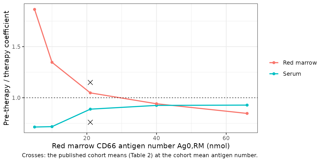

6. Immunoreactivity matters

The paper’s other claim is that assuming r_im = 1 is untenable. Setting r_im = 1 removes the half and non-immunoreactive circulations entirely and should visibly change the biodistribution.

modPerfect <- rxode2::rxode2(rxode2::ini(readModelDb("Kletting_2015_antiCD66_pbpk_model1"),
                                         rIm = 1))
#> ℹ change initial estimate of `rIm` to `1`
prePerfect <- solveOne(modPerfect, abPt, tmaxTiac)

tibble::tibble(
  Organ = unname(cols),
  `r_im = 0.801 (fitted)` = vals["m1", ],
  `r_im = 1 (the abandoned assumption)` =
    vapply(names(cols), function(cc) tiac(prePerfect, cc, labPt), 0),
  `Paper pre-therapy` = c("42.2 +/- 7.7", "6.6 +/- 2.1", "3.1 +/- 1.3",
                          "3.8 +/- 1.4", "72.4 +/- 3.4")
) |>
  knitr::kable(digits = 2)

Organ	r_im = 0.801 (fitted)	r_im = 1 (the abandoned assumption)	Paper pre-therapy
Red marrow	44.93	58.85	42.2 +/- 7.7
Liver	5.63	2.81	6.6 +/- 2.1
Spleen	2.61	1.53	3.1 +/- 1.3
Serum [h/L]	3.04	0.73	3.8 +/- 1.4
Whole body	73.87	70.52	72.4 +/- 3.4

# Perfect immunoreactivity moves more antibody onto antigen and less into serum.
stopifnot(tiac(prePerfect, "Cc", labPt) < tiac(pre1, "Cc", labPt),
          tiac(prePerfect, "abMarrow", labPt) > tiac(pre1, "abMarrow", labPt))

# And it must fail the Table 2 gate that the fitted r_im passes: the serum
# coefficient collapses to a fifth of the published value and the red marrow
# coefficient lands more than two between-patient SDs high.
stopifnot(tiac(prePerfect, "Cc", labPt) < 0.25 * 3.8,
          (tiac(prePerfect, "abMarrow", labPt) - 42.2) / 7.7 > 2)

With r_im = 1 the red marrow coefficient rises to about 59 h against the published 42.2 +/- 7.7 h and the serum coefficient collapses from 3.0 to 0.7 h/L against the published 3.8 +/- 1.4. Both miss badly, which is the paper’s reason for abandoning the assumption.

Assumptions and deviations

• Three printed equations are encoded against their printed form. Each is a transcription slip contradicted by the equation’s own labelled twin, by the prose it follows, or by mass balance:
  • S1 Text Eq 8 and Eq 9 print Ag0,B = (Ag0,L + Ag0,S) * 0.9. The sentence immediately above states that the liver and spleen cells equal 90 % of the circulating pool, which is division, and Table 1’s means are a linear map of the fitted pair: Ag0,L 0.31 + Ag0,S 0.22 = 0.53 against the reported Ag0,B 0.58. Division gives 0.589 and multiplication 0.477, so the constraint is encoded as / 0.9. Printed Eqs 6 and 7 are inverted in the same way relative to their own prose.
  • S1 Text Eq 35, the unlabelled non-immunoreactive spleen and marrow equation, prints a minus on the inflow from the main vascular compartment. Its own labelled twin on the next line and Eq 36 both print a plus, and a minus would make the compartment a sink; encoded positive.
  • S1 Text Eq 39, the unlabelled non-immunoreactive vascular equation, picks up k_out * Ab_ha,int and lambda_phy * Ab*_ha,P from the half immunoreactive Eq 34. Its labelled twin uses the na states; encoded as na.
• Eq 29 carries two fully-immunoreactive terms that a half immunoreactive antibody cannot have. As printed it includes - k_on,mono * alpha_i * Ag_i * AgAb_ha,mono and + 2 k_off * AgAb_ha,bi, both crosslinking terms. There is no AgAb_ha,bi state anywhere in the supplement, Eq 2’s antigen balance has no half immunoreactive bivalent term, and the paper defines half immunoreactive antibody as having one active arm, so it cannot crosslink. Keeping the alpha loss would drain bound antibody into a compartment that does not exist and break mass balance; both terms are dropped. The printed factor 2 on the half immunoreactive association rate is kept as published, even though the model’s own arm-counting bookkeeping (two free arms give 2 k_on,mono for the fully immunoreactive species) would imply 1 for a one-armed antibody. It is internally consistent between Eqs 29 and 30, it conserves mass, and it is what the authors’ SAAM II implementation presumably contained when the shipped parameters were fitted.
• alpha_i needs a unit conversion the supplement does not print. Table B gives alpha_i in 1/cm3 and k_on,mono in L/nmol/min, so the product k_on,mono * alpha_i * Ag_i is short by a factor of 1000. The model applies it explicitly. The reading is confirmed independently: computing k_on,bi * [Ag]_s from Table B’s E, r_cell and N_cells,RM gives the same 35 /min crosslinking rate at the cohort-mean antigen number.
• The whole-body observable has no printed equation. S1 Text gives data-assignment equations for liver, spleen, serum and red marrow (Eqs 17-21) but not for the whole-body gamma-camera signal. It is encoded as every radiolabelled state that has not yet been excreted, which is the only reading consistent with a whole-body count, and it reproduces Table 2’s 72.4 h and stays below the 96.9 h physical bound.
• cleared_lab and cleared_unlab are bookkeeping states, not published ones. They accumulate the lambda_cl outflow so that total antibody mass is exactly conserved and the mass-balance gate above is possible. They enter no other equation.
• Model 2’s organ-size weights are shipped as parameters fixed at 1. Eq 9 weights each organ’s antigen number by V_MRI / V_Cal. Neither the per-patient MRI volumes nor the formulae for the calculated volumes (refs [9] Harris 2010 and [10] Johnson 2005) appear in any on-disk source, so the ratios themselves are the shipped input (ratioVolLiver, ratioVolSpleen), fixed at 1 = an organ of exactly calculated size. At that default Model 2 reduces to Model 1’s constraint and differs only through its own column of Table 1 estimates, which is what this vignette’s model averaging uses. A user with measured volumes overrides them with rxode2::ini().
• No inter-individual variability is encoded. The paper fitted 27 patients individually; Table 1’s SDs are spreads of individual estimates inflated by estimation error, not a fitted omega. They are recorded in population$notes.
• The radiolabelled fraction and the physical decay constant are model parameters, not covariates. fracLabeled and lambdaPhy differ between the 111In tracer and the 90Y therapy administration and are switched with rxode2::ini() between the two solves above. The shipped values are the tracer’s, the data the parameters were fitted to.
• The residual 111In-labelled antibody is folded into the unlabelled pool at the therapy injection. It is chemically the same antibody and still occupies antigen, but a 90Y measurement cannot see it. Folding costs the small difference between the two decay constants (1.72e-4 against 1.80e-4 /min, 4.6 %) applied to 7.5 % of a dose that is itself a quarter of the therapy dose.
• Residual antibody at therapy is larger here than the Discussion’s rounded figure. The model leaves 34 % of the tracer’s antibody in the body at 192 h against the paper’s “~20 % unlabelled”. The interval between the two administrations is not tabulated per patient – 192 h is read off patient 1’s first 90Y serum sample in S1 Table – and a longer interval in other patients would lower the figure. The radiolabelled residual matches: the model gives 7.5 % of injected activity against the paper’s “~8 %”. Nothing was tuned.
• Demographics are assumed. The paper reports no age, sex, weight or height distribution. WT = 70 kg and HT = 170 cm are the reference adult; HT = 170 makes the UlmDos factor K = 1 / 0.06665 exactly. WT affects only the bivalent enhancement factor through the cell numbers and HT only the abMarrowRoi readout, so neither touches the coefficients validated above.
• Table 2 is reproduced at typical parameters, not patient by patient. The published coefficients are means over 27 individual fits; the model here is solved once at the Table 1 means. The two agree within one between-patient SD on every organ, but ratios that depend non-linearly on the antigen number (Section 5) are understated at mean parameters, as the sweep shows.