Veliparib and its M8 metabolite (Niu 2017)
Source:vignettes/articles/Niu_2017_veliparib.Rmd
Niu_2017_veliparib.RmdModel and source
#> ℹ parameter labels from comments will be replaced by 'label()'Citation: Niu J., Scheuerell C., Mehrotra S., Karan S., Puhalla S., Kiesel B. F., Ji J., Chu E., Gopalakrishnan M., Ivaturi V., Gobburu J., Beumer J. H. (2017). Parent-metabolite pharmacokinetic modeling and pharmacodynamics of veliparib (ABT-888), a PARP inhibitor, in patients with BRCA 1/2-mutated cancer or PARP-sensitive tumor types. The Journal of Clinical Pharmacology 57(8):977-987. doi:10.1002/jcph.892.
Description: Joint parent plus metabolite population PK model for the oral PARP inhibitor veliparib (ABT-888) and its primary active metabolite M8, in patients with BRCA 1/2-mutated cancer or PARP-sensitive tumor types. Veliparib disposition is two-compartment with first-order absorption and an absorption lag time; total apparent clearance CL/F is split into a renal arm CLR/F = CL/F * frenal, which is a power function of Cockcroft-Gault creatinine clearance, and a non-renal arm CLNR/F = CL/F * fm, which is the formation clearance that is assumed to produce all of the M8. M8 is described by a two-compartment model with first-order formation. Lean body mass enters as a power function on the veliparib central volume of distribution. The renal and metabolised fractions were not identifiable from these data and were held at frenal = 0.7 and fm = 1 - frenal = 0.3 from a published mass-balance study.
Article: https://doi.org/10.1002/jcph.892
Niu 2017 fitted veliparib (ABT-888) and its primary active metabolite
M8 simultaneously in a single joint model, so this
paper contributes one model file (Niu_2017_veliparib)
rather than a separate parent and metabolite model.
The structure, reproduced from Niu 2017 Figure 1, is:
                 Parent Periph.          M8 Periph.
                     Vp/F                  Vp_met
                       ^                      ^
                  Q/F  |                 Qmet |
                       v                      v
  Dose --Ka,tlag--> Parent Central --------> M8 Central
                     Vc/F        CLNR/F        Vc_met
                       |        = CL/F*fm        |
                CLR/F  |                         | CLmet
             = CL/F *  v                         v
             frenal *
             (CLCR/95)^p
The single estimated total apparent clearance CL/F is
split into a renal arm (CLR/F, the only arm carrying the
creatinine-clearance covariate) and a non-renal arm
(CLNR/F), which is the formation clearance feeding M8. The
two arms carry separate between-subject random effects,
which is what Table 2’s distinct omega CLR/F and
omega CLNR/F rows report.
Population
The model was developed from a phase 1 multicentre, randomised, open-label dose-escalation study of chronically dosed single-agent veliparib in patients with BRCA 1/2-mutated cancer or PARP-sensitive tumour types (ClinicalTrials.gov NCT00892736). Seventy-one patients were enrolled; 67 contributed veliparib pharmacokinetic samples and form the modelled population, of whom 38 also contributed M8 samples. A further 41 patients contributed 295 PAR measurements in peripheral blood mononuclear cells for the exploratory pharmacodynamic analysis. In total 1214 veliparib and 656 M8 plasma concentrations were fitted.
The cohort was almost entirely female (69/71, 97%), consistent with a BRCA-enriched breast and ovarian cancer population, with mean age 53.5 years (range 28.0-84.0), mean total body weight 74.9 kg (45.0-119), mean lean body mass 47.6 kg (36.6-63.7) and mean Cockcroft-Gault creatinine clearance 95.2 mL/min (48.5-120). ECOG performance status was 0 in 61%, 1 in 31% and 2 in 8%. Patients were treated at one of nine AM/PM dose levels from 50/50 to 500/500 mg twice daily; only the morning dose was given on day 1, with twice-daily dosing from day 2 (Niu 2017 Table 1 and Methods “Subjects, Study Design, and Treatment”).
Two data-handling rules from Table 1’s footnote are part of the fitted model and are reproduced in the virtual cohort below: Cockcroft-Gault CLCR estimates above 120 mL/min were assigned 120 mL/min (this affected 20 of the 71 patients), and the covariate centring constants are the cohort central values, 95 mL/min for CLCR and 48 kg for LBM.
The same information is available programmatically via
readModelDb("Niu_2017_veliparib")()$population.
Source trace
The per-parameter origin is recorded as an in-file comment next to
each ini() entry in
inst/modeldb/specificDrugs/Niu_2017_veliparib.R. The table
below collects them in one place for review.
| Equation / parameter | Value | Source location |
|---|---|---|
| Model structure (2-cmt parent + 2-cmt metabolite, first-order absorption with lag) | n/a | Figure 1; Results paragraphs 2-3 |
lka (Ka) |
2.02 1/h | Table 2 |
ltlag (tlag) |
0.272 h | Table 2 |
lvc (Vc/F) |
99.2 L | Table 2 |
lvp (Vp/F) |
47.8 L | Table 2 |
lq (Q/F) |
17.9 L/h | Table 2 |
lcl (CL/F) |
17.3 L/h | Table 2 |
fm |
0.3 (held) | Table 2 “fm 0.3 (fix)”; Figure 1 legend
fm = 1 - frenal
|
frenal (derived as 1 - fm) |
0.7 (held) | Table 2 “frenal 0.7 (fix)”; Methods “Base Model” |
lvc_m8 (Vc_met) |
23.6 L | Table 2 |
lvp_m8 (Vp_met) |
51.4 L | Table 2 |
lq_m8 (Qmet) |
29.0 L/h | Table 2 |
lcl_m8 (CLmet) |
22.8 L/h | Table 2 |
e_lbm_vc (power_LBM) |
1.21 | Table 2; Equation 7 |
e_crcl_cl_renal (power_CLcr) |
0.903 | Table 2; Equation 5 |
CLR/F = CL/F * frenal * (CLCR/95)^p |
n/a | Equation 5 |
CLNR/F = CL/F * fm |
n/a | Equation 6 |
Vc/F = Vc/F * (LBM/48)^p |
n/a | Equation 7 |
IIV, exponential theta * exp(eta)
|
n/a | Equation 1 |
| Covariate form, median-centred power | n/a | Equation 3 |
etalka .. etalcl_m8 (9 variances) |
Table 2 CV% squared | Table 2 “Between-subject variability” |
| No IIV on Q, Qmet | n/a | Results; Supplemental Table S1 runs 112, 113 |
| No IIV correlation block | n/a | Results (dropped: condition number 1e8) |
propSd (veliparib) |
0.251 | Table 2 “CMultStdev 25.1%” |
addSd (veliparib) |
0.607 ng/mL | Table 2 |
propSd_m8 |
0.251 * 0.808 * 1.00 = 0.202808 | Table 2 notes (CMultStdev * Ratio * MultStdev) |
addSd_m8 |
3.37 ng/mL | Table 2 |
| Population metadata | n/a | Table 1; Results paragraph 1 |
| Unit convention (ng/mL, no MW correction) | n/a | Methods “Software and Estimation Methods” |
Structural verification
Before any stochastic simulation, the packaged model is checked
against closed forms that follow from the published equations. These use
zeroRe() so both sides of every comparison use the
same parameter values – the residual difference is pure
ODE-solver error, so tight bounds are appropriate here (and are
deliberately not used for the Monte Carlo checks further down).
mod  <- readModelDb("Niu_2017_veliparib")
modz <- rxode2::zeroRe(rxode2::rxode(mod))
#> ℹ parameter labels from comments will be replaced by 'label()'

# Event table helper. Observation rows carry the ODE-state name in `cmt` plus
# `dvid = 1L`; the model has two endpoints (Cc, Cc_m8) so rxode2 needs the
# endpoint disambiguated. Both observables are returned as columns regardless.
mk_events <- function(dose, times, LBM = 48, CRCL = 95, id = 1L,
                      dose_times = 0) {
  dplyr::bind_rows(
    data.frame(id = id, time = dose_times, amt = dose, evid = 1L,
               cmt = "depot", dvid = NA_integer_),
    data.frame(id = id, time = times, amt = NA_real_, evid = 0L,
               cmt = "central", dvid = 1L)
  ) |>
    dplyr::mutate(LBM = LBM, CRCL = CRCL) |>
    dplyr::arrange(id, time, dplyr::desc(evid))
}

solve_typ <- function(ev) {
  rxode2::rxSolve(modz, ev, returnType = "data.frame",
                  useLinCmt = FALSE, atol = 1e-12, rtol = 1e-12)
}

trapz <- function(x, y) sum(diff(x) * (utils::head(y, -1) + utils::tail(y, -1)) / 2)

# A window of ~110 terminal half-lives is not useful (the tail decays into
# solver noise); the parent terminal half-life is about 6.6 h, so 720 h is used
# only for these closed-form AUC checks where high accuracy is wanted, and the
# NCA below uses a 120 h (about 18 half-life) window instead.
tgrid <- seq(0, 720, by = 0.05)
ref   <- solve_typ(mk_events(400, tgrid))
#> ℹ omega/sigma items treated as zero: 'etalka', 'etaltlag', 'etalvc', 'etalvp', 'etalcl_renal', 'etalcl_nonren', 'etalvc_m8', 'etalvp_m8', 'etalcl_m8'

structural <- tibble::tibble(
  Quantity = c(
    "Vc/F at LBM = 48 kg (L)",
    "CLR/F at CLCR = 95 mL/min (L/h)",
    "CLNR/F (L/h)",
    "Total CL/F (L/h)",
    "Veliparib AUC(0-inf) after 400 mg (ng*h/mL)",
    "M8 AUC(0-inf) after 400 mg (ng*h/mL)"
  ),
  Simulated = c(ref$vc[1], ref$cl_renal[1], ref$cl_nonren[1],
                ref$cl_renal[1] + ref$cl_nonren[1],
                trapz(ref$time, ref$Cc), trapz(ref$time, ref$Cc_m8)),
  `Closed form` = c(
    99.2,                        # Table 2 Vc/F, since (48/48)^1.21 = 1
    17.3 * 0.7,                  # Eq. 5 at the centring value
    17.3 * 0.3,                  # Eq. 6
    17.3,                        # Table 2 CL/F
    1000 * 400 / 17.3,           # Dose / CL, x1000 ng per ug
    1000 * 400 * 0.3 / 22.8      # Dose * fm / CLmet
  ),
  check.names = FALSE
) |>
  dplyr::mutate(`% diff` = 100 * (Simulated - `Closed form`) / `Closed form`)

knitr::kable(structural, digits = c(0, 4, 4, 5),
caption = "Packaged model against closed forms derived from Niu 2017 Equations 5-7 and Table 2.")| Quantity | Simulated | Closed form | check.names | % diff |
|---|---|---|---|---|
| Vc/F at LBM = 48 kg (L) | 99.200 | 99.200 | FALSE | 0 |
| CLR/F at CLCR = 95 mL/min (L/h) | 12.110 | 12.110 | FALSE | 0 |
| CLNR/F (L/h) | 5.190 | 5.190 | FALSE | 0 |
| Total CL/F (L/h) | 17.300 | 17.300 | FALSE | 0 |
| Veliparib AUC(0-inf) after 400 mg (ng*h/mL) | 23122.193 | 23121.387 | FALSE | 0 |
| M8 AUC(0-inf) after 400 mg (ng*h/mL) | 5263.158 | 5263.158 | FALSE | 0 |
The two AUC identities are the load-bearing checks.
AUC = Dose / CL confirms the parent mass balance, and
AUC_M8 = Dose * fm / CLmet confirms that the formation flux
out of the parent central compartment arrives in the M8 central
compartment intact – i.e. that the CLNR/F arm is wired to
the metabolite and not to an elimination sink.
Three further structural properties the paper asserts:
auc_ref <- trapz(ref$time, ref$Cc)

# (a) Dose proportionality from 50 to 500 mg (Niu 2017 Discussion: "Dose
#     proportionality in dose level from 50 to 500 mg was supported here").
dose_prop <- vapply(c(50, 100, 200, 300, 400, 500), function(d) {
  s <- solve_typ(mk_events(d, tgrid))
  trapz(s$time, s$Cc) / d
}, numeric(1))
#> ℹ omega/sigma items treated as zero: 'etalka', 'etaltlag', 'etalvc', 'etalvp', 'etalcl_renal', 'etalcl_nonren', 'etalvc_m8', 'etalvp_m8', 'etalcl_m8'
#> ℹ omega/sigma items treated as zero: 'etalka', 'etaltlag', 'etalvc', 'etalvp', 'etalcl_renal', 'etalcl_nonren', 'etalvc_m8', 'etalvp_m8', 'etalcl_m8'
#> ℹ omega/sigma items treated as zero: 'etalka', 'etaltlag', 'etalvc', 'etalvp', 'etalcl_renal', 'etalcl_nonren', 'etalvc_m8', 'etalvp_m8', 'etalcl_m8'
#> ℹ omega/sigma items treated as zero: 'etalka', 'etaltlag', 'etalvc', 'etalvp', 'etalcl_renal', 'etalcl_nonren', 'etalvc_m8', 'etalvp_m8', 'etalcl_m8'
#> ℹ omega/sigma items treated as zero: 'etalka', 'etaltlag', 'etalvc', 'etalvp', 'etalcl_renal', 'etalcl_nonren', 'etalvc_m8', 'etalvp_m8', 'etalcl_m8'
#> ℹ omega/sigma items treated as zero: 'etalka', 'etaltlag', 'etalvc', 'etalvp', 'etalcl_renal', 'etalcl_nonren', 'etalvc_m8', 'etalvp_m8', 'etalcl_m8'

# (b) LBM acts on Vc/F only, so it must move Cmax but NOT AUC.
lbm_hi  <- solve_typ(mk_events(400, tgrid, LBM = 60))
#> ℹ omega/sigma items treated as zero: 'etalka', 'etaltlag', 'etalvc', 'etalvp', 'etalcl_renal', 'etalcl_nonren', 'etalvc_m8', 'etalvp_m8', 'etalcl_m8'
lbm_vc  <- lbm_hi$vc[1]

# (c) M8-to-parent exposure ratio = fm * CL/F / CLmet.
ratio_sim <- trapz(ref$time, ref$Cc_m8) / auc_ref

tibble::tibble(
  Property = c("AUC/dose constant over 50-500 mg (max spread, %)",
               "Vc/F at LBM = 60 kg vs 99.2*(60/48)^1.21 (% diff)",
               "AUC change when LBM 48 -> 60 kg (%)",
               "M8:parent AUC ratio vs fm*CL/CLmet (% diff)"),
  Value = c(
    100 * (max(dose_prop) - min(dose_prop)) / mean(dose_prop),
    100 * (lbm_vc - 99.2 * (60 / 48)^1.21) / (99.2 * (60 / 48)^1.21),
    100 * (trapz(lbm_hi$time, lbm_hi$Cc) - auc_ref) / auc_ref,
    100 * (ratio_sim - 0.3 * 17.3 / 22.8) / (0.3 * 17.3 / 22.8)
  )
) |>
knitr::kable(digits = 5, caption = "Further structural properties.")| Property | Value |
|---|---|
| AUC/dose constant over 50-500 mg (max spread, %) | 0.00000 |
| Vc/F at LBM = 60 kg vs 99.2*(60/48)^1.21 (% diff) | 0.00000 |
| AUC change when LBM 48 -> 60 kg (%) | -0.00082 |
| M8:parent AUC ratio vs fm*CL/CLmet (% diff) | -0.00347 |
stopifnot(
  100 * (max(dose_prop) - min(dose_prop)) / mean(dose_prop) < 0.01,
  abs(lbm_vc - 99.2 * (60 / 48)^1.21) < 1e-8,
  abs(trapz(lbm_hi$time, lbm_hi$Cc) - auc_ref) / auc_ref < 1e-4,
  abs(ratio_sim - 0.3 * 17.3 / 22.8) < 1e-4
)
Renal-function covariate: a discrepancy inside the paper
Niu 2017 Discussion states: “According to our covariate model, patients with mild (~25% decrease in CLCR) and moderate (~50% decrease in CLCR) renal function are associated with ~10% and ~20% increase in veliparib exposure, respectively.” That sentence is not reproducible from the paper’s own Equation 5, and the table below shows why. Because Equation 5, Figure 1 and Table 2 all agree with each other and only the Discussion prose disagrees, the equation is what the model file encodes.
renal <- lapply(c(1.00, 0.75, 0.50), function(f) {
  crcl <- 95 * f
  s <- solve_typ(mk_events(400, tgrid, CRCL = crcl))
  tibble::tibble(
    `CLCR (mL/min)` = crcl,
    `Change in CLCR (%)` = 100 * (f - 1),
    `CL/F (L/h)` = s$cl_renal[1] + s$cl_nonren[1],
    `CL/F closed form` = 17.3 * 0.7 * (crcl / 95)^0.903 + 17.3 * 0.3,
    `Exposure increase (%)` = 100 * (trapz(s$time, s$Cc) / auc_ref - 1)
  )
}) |> dplyr::bind_rows()
#> ℹ omega/sigma items treated as zero: 'etalka', 'etaltlag', 'etalvc', 'etalvp', 'etalcl_renal', 'etalcl_nonren', 'etalvc_m8', 'etalvp_m8', 'etalcl_m8'
#> ℹ omega/sigma items treated as zero: 'etalka', 'etaltlag', 'etalvc', 'etalvp', 'etalcl_renal', 'etalcl_nonren', 'etalvc_m8', 'etalvp_m8', 'etalcl_m8'
#> ℹ omega/sigma items treated as zero: 'etalka', 'etaltlag', 'etalvc', 'etalvp', 'etalcl_renal', 'etalcl_nonren', 'etalvc_m8', 'etalvp_m8', 'etalcl_m8'

renal$`Paper Discussion claims (%)` <- c(0, 10, 20)

knitr::kable(renal, digits = 3,
caption = "Equation 5 reproduced exactly, against the exposure claim in the paper's Discussion.")| CLCR (mL/min) | Change in CLCR (%) | CL/F (L/h) | CL/F closed form | Exposure increase (%) | Paper Discussion claims (%) |
|---|---|---|---|---|---|
| 95.00 | 0 | 17.300 | 17.300 | 0.000 | 0 |
| 71.25 | -25 | 14.530 | 14.530 | 19.067 | 10 |
| 47.50 | -50 | 11.666 | 11.666 | 48.291 | 20 |
# The equation is reproduced exactly; that is what is asserted.
stopifnot(all(abs(renal$`CL/F (L/h)` - renal$`CL/F closed form`) < 1e-8))
The implemented model gives a +19.1% and
+48.3% exposure increase for a 25% and 50% fall in
CLCR, against the Discussion’s “~10%” and “~20%”. Note the arithmetic is
straightforward and does not depend on this implementation: at CLCR =
71.25 mL/min, Equation 5 gives
CLR/F = 17.3 * 0.7 * 0.75^0.903 = 9.34 L/h, so
CL/F = 9.34 + 5.19 = 14.53 L/h and the exposure ratio is
17.3 / 14.53 = 1.19. Because the non-renal arm is only 30%
of total clearance, a renal-arm exponent near 1 necessarily produces an
exposure change substantially larger than the Discussion’s figures. See
“Assumptions and deviations” below.
Virtual cohort
Original observed data are not publicly available. The cohort below approximates the Table 1 demographics: lean body mass and Cockcroft-Gault creatinine clearance are drawn to match the reported means and ranges, and CLCR is capped at 120 mL/min exactly as the paper did before estimation.
Three of the nine studied dose levels are simulated, spanning the range: 50/50, 200/200 and 400/400 mg. 100 subjects per arm is well inside the 200/arm cap.
set.seed(20170808)
n_per_arm <- 100L
dose_levels <- c(50, 200, 400)

# Sampling grid, out to 120 h (about 18 parent terminal half-lives -- long
# enough for AUC(0-inf) extrapolation, short enough that the tail has not
# decayed into solver noise). The absorption phase is sampled at 0.05 h
# because IIV on Ka is large (omega = 0.781): the fastest-absorbing subjects
# peak well before the population tmax of about 1.4 h, and a 0.25 h grid
# under-resolves their peak badly enough to cost 0.9% on the AUC = Dose/CL
# identity asserted below. At 0.05 h that error drops to below 0.05%.
obs_times <- sort(unique(c(
  seq(0, 6, by = 0.05), seq(6, 24, by = 0.25), seq(25, 120, by = 1)
)))

make_cohort <- function(n, dose, id_offset = 0L) {
  subj <- tibble::tibble(
    id = id_offset + seq_len(n),
    # Table 1 (Total): LBM mean 47.6 kg, range 36.6-63.7.
    LBM = pmin(pmax(stats::rnorm(n, mean = 47.6, sd = 5.2), 36.6), 63.7),
    # Table 1 (Total): CLCR mean 95.2 mL/min, range 48.5-120, capped at 120.
    CRCL = pmin(pmax(stats::rnorm(n, mean = 95.2, sd = 17.5), 48.5), 120),
    treatment = paste0(dose, " mg")
  )
  dplyr::bind_rows(
    subj |> dplyr::mutate(time = 0, amt = dose, evid = 1L,
                          cmt = "depot", dvid = NA_integer_),
    tidyr::crossing(subj, time = obs_times) |>
      dplyr::mutate(amt = NA_real_, evid = 0L, cmt = "central", dvid = 1L)
  ) |>
    dplyr::arrange(id, time, dplyr::desc(evid))
}

events <- dplyr::bind_rows(
  lapply(seq_along(dose_levels), function(i) {
    make_cohort(n_per_arm, dose_levels[i], id_offset = (i - 1L) * n_per_arm)
  })
)

stopifnot(!anyDuplicated(unique(events[, c("id", "time", "evid")])))
Simulation
sim <- rxode2::rxSolve(
  mod, events = events,
  keep = c("treatment"),
  useLinCmt = FALSE
) |>
  as.data.frame()
#> ℹ parameter labels from comments will be replaced by 'label()'

# No solver artefacts in the tail before NCA sees them.
stopifnot(all(sim$Cc >= 0, na.rm = TRUE), all(sim$Cc_m8 >= 0, na.rm = TRUE))
Single-dose concentration-time profiles
Replicates the shape of Supplemental Figure S1 (left panels, day 1 of cycle 1), which plots mean veliparib and M8 plasma concentration versus time after the morning dose by dose level. Only the morning dose was given on day 1, so the day-1 data are a single-dose profile.
sim |>
  dplyr::filter(time <= 24) |>
  dplyr::select(id, time, treatment, Veliparib = Cc, M8 = Cc_m8) |>
  tidyr::pivot_longer(c(Veliparib, M8), names_to = "Analyte",
                      values_to = "conc") |>
  dplyr::mutate(Analyte = factor(Analyte, levels = c("Veliparib", "M8"))) |>
  dplyr::group_by(time, treatment, Analyte) |>
  dplyr::summarise(mean_conc = mean(conc), .groups = "drop") |>
  ggplot(aes(time, mean_conc, colour = treatment)) +
  geom_line(linewidth = 0.7) +
  facet_wrap(~Analyte, scales = "free_y") +
  scale_x_continuous(breaks = seq(0, 24, by = 4)) +
  labs(x = "Time after morning dose (h)", y = "Mean concentration (ng/mL)",
       colour = "Dose level",
       title = "Day 1, cycle 1: mean concentration-time profiles",
       caption = "Replicates Supplemental Figure S1 (left panels) of Niu 2017.") +
  theme_bw()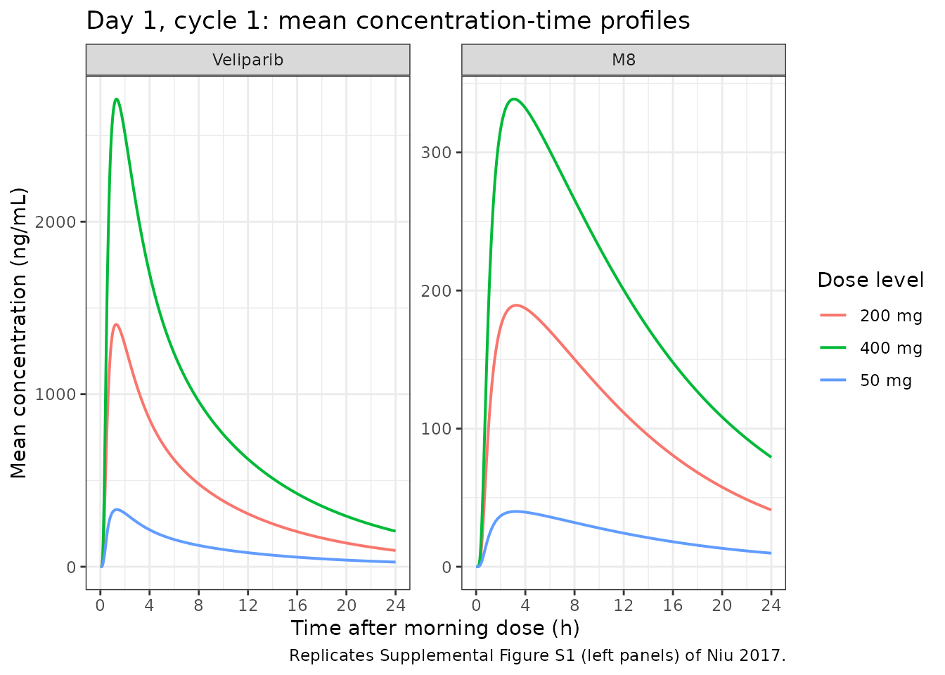
Prediction interval
Replicates the presentation of Figure 4 (visual predictive check), showing the 5th, 50th and 95th percentiles of the simulated profiles. Niu 2017 has no digitised observed data available here, so this shows the model’s own predictive distribution rather than an overlay.
sim |>
  dplyr::filter(time <= 24) |>
  dplyr::select(id, time, treatment, Veliparib = Cc, M8 = Cc_m8) |>
  tidyr::pivot_longer(c(Veliparib, M8), names_to = "Analyte",
                      values_to = "conc") |>
  dplyr::mutate(Analyte = factor(Analyte, levels = c("Veliparib", "M8"))) |>
  dplyr::group_by(time, treatment, Analyte) |>
  dplyr::summarise(
    Q05 = stats::quantile(conc, 0.05),
    Q50 = stats::quantile(conc, 0.50),
    Q95 = stats::quantile(conc, 0.95),
    .groups = "drop"
  ) |>
  ggplot(aes(time, Q50)) +
  geom_ribbon(aes(ymin = Q05, ymax = Q95), alpha = 0.25) +
  geom_line(linewidth = 0.7) +
  facet_grid(Analyte ~ treatment, scales = "free_y") +
  labs(x = "Time after morning dose (h)", y = "Concentration (ng/mL)",
       title = "Simulated 5th / 50th / 95th percentiles, day 1",
       caption = "Presentation follows Figure 4 of Niu 2017.") +
  theme_bw()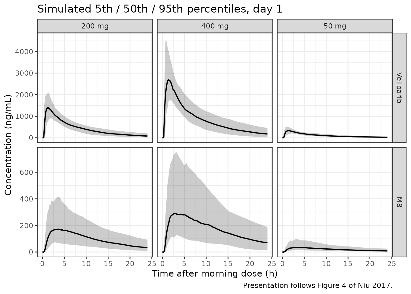
PKNCA validation
One PKNCA block per output, as the model has two.
nca_input <- function(conc_col) {
  d <- sim |>
    dplyr::filter(!is.na(.data[[conc_col]])) |>
    dplyr::select(id, time, treatment, Cc = dplyr::all_of(conc_col))
  # Guarantee a time = 0 row per subject; pre-dose Cc = 0 is correct for an
  # extravascular dose. Existing time = 0 rows win.
  dplyr::bind_rows(
    d,
    d |> dplyr::distinct(id, treatment) |> dplyr::mutate(time = 0, Cc = 0)
  ) |>
    dplyr::distinct(id, treatment, time, .keep_all = TRUE) |>
    dplyr::arrange(id, treatment, time)
}

dose_df <- events |>
  dplyr::filter(evid == 1) |>
  dplyr::select(id, time, amt, treatment)

dose_obj <- PKNCA::PKNCAdose(dose_df, amt ~ time | treatment + id,
                             doseu = "mg")

intervals <- data.frame(
  start = 0, end = Inf,
  cmax = TRUE, tmax = TRUE, aucinf.obs = TRUE, half.life = TRUE,
  cl.obs = TRUE
)

run_nca <- function(conc_col) {
  conc_obj <- PKNCA::PKNCAconc(nca_input(conc_col), Cc ~ time | treatment + id,
                               concu = "ng/mL", timeu = "h")
  PKNCA::pk.nca(PKNCA::PKNCAdata(conc_obj, dose_obj, intervals = intervals))
}

nca_parent <- run_nca("Cc")
nca_m8     <- run_nca("Cc_m8")
Per-subject identities
The strongest available check: for every simulated subject, the NCA-derived exposure must reproduce that subject’s own drawn clearances. Both sides use the same realised parameters, so these are exact identities and are asserted tightly.
subj_par <- sim |>
  dplyr::group_by(id, treatment) |>
  dplyr::summarise(cl_renal = dplyr::first(cl_renal),
                   cl_nonren = dplyr::first(cl_nonren),
                   cl_m8 = dplyr::first(cl_m8),
                   .groups = "drop") |>
  dplyr::mutate(cl_total = cl_renal + cl_nonren) |>
  dplyr::left_join(dose_df |> dplyr::select(id, amt), by = "id")

auc_of <- function(res) {
  as.data.frame(res$result) |>
    dplyr::filter(PPTESTCD == "aucinf.obs") |>
    dplyr::select(id, auc = PPORRES)
}

ident <- subj_par |>
  dplyr::left_join(auc_of(nca_parent) |> dplyr::rename(auc_p = auc), by = "id") |>
  dplyr::left_join(auc_of(nca_m8)     |> dplyr::rename(auc_m = auc), by = "id") |>
  dplyr::mutate(
    # AUC(0-inf) = 1000 * Dose / CL_total
    pred_p = 1000 * amt / cl_total,
    # AUC_M8(0-inf) = 1000 * Dose * CLNR / (CL_total * CLmet)
    pred_m = 1000 * amt * cl_nonren / (cl_total * cl_m8),
    err_p = 100 * (auc_p - pred_p) / pred_p,
    err_m = 100 * (auc_m - pred_m) / pred_m
  )

stopifnot(nrow(ident) == n_per_arm * length(dose_levels), !anyNA(ident$err_p),
          !anyNA(ident$err_m))

tibble::tibble(
  Identity = c("Veliparib AUC(0-inf) = 1000 * Dose / CL/F",
               "M8 AUC(0-inf) = 1000 * Dose * CLNR/F / (CL/F * CLmet)"),
  `n subjects` = nrow(ident),
  `max |% error|` = c(max(abs(ident$err_p)), max(abs(ident$err_m)))
) |>
  knitr::kable(digits = 4,
caption = "Per-subject exact identities across the whole cohort.")| Identity | n subjects | max |% error| |
|---|---|---|
| Veliparib AUC(0-inf) = 1000 * Dose / CL/F | 300 | 0.0434 |
| M8 AUC(0-inf) = 1000 * Dose * CLNR/F / (CL/F * CLmet) | 300 | 0.0166 |
# Bound set just above the accuracy actually achieved on this sampling grid
# (parent 0.043%, M8 0.017%), so it catches a regression rather than merely
# passing. The residual is trapezoidal error in the absorption phase, not
# model error: both sides use the same realised parameters.
stopifnot(max(abs(ident$err_p)) < 0.1, max(abs(ident$err_m)) < 0.1)
Comparison against published values
Niu 2017 reports no NCA table of its own, but it reports the final
model’s typical CL/F (Table 2) and, in the Discussion, an
external NCA comparator for CL/F from an earlier veliparib
study (reference 23; 18 L/h). The comparison below is run on a
typical-value subject at the reference covariates
(zeroRe(), LBM 48 kg, CLCR 95 mL/min), so the simulated
side is the model’s own typical prediction and the comparison is exact
rather than Monte Carlo.
# Each dose level is a separate single-subject solve. A typical-value cohort has
# exactly one subject per scenario -- bundling the three dose levels into one
# multi-subject solve would add nothing and makes rxode2 warn that a
# multi-subject simulation carries no omega (which is the whole point of
# zeroRe()).
typ_events <- lapply(seq_along(dose_levels), function(i) {
  mk_events(dose_levels[i], obs_times, id = i) |>
    dplyr::mutate(treatment = paste0(dose_levels[i], " mg"))
})

sim_typ <- lapply(typ_events, function(ev) {
  rxode2::rxSolve(modz, ev, keep = c("treatment"), useLinCmt = FALSE) |>
    as.data.frame() |>
    dplyr::mutate(id = ev$id[1])
}) |>
  dplyr::bind_rows()
#> ℹ omega/sigma items treated as zero: 'etalka', 'etaltlag', 'etalvc', 'etalvp', 'etalcl_renal', 'etalcl_nonren', 'etalvc_m8', 'etalvp_m8', 'etalcl_m8'
#> ℹ omega/sigma items treated as zero: 'etalka', 'etaltlag', 'etalvc', 'etalvp', 'etalcl_renal', 'etalcl_nonren', 'etalvc_m8', 'etalvp_m8', 'etalcl_m8'
#> ℹ omega/sigma items treated as zero: 'etalka', 'etaltlag', 'etalvc', 'etalvp', 'etalcl_renal', 'etalcl_nonren', 'etalvc_m8', 'etalvp_m8', 'etalcl_m8'

typ_events <- dplyr::bind_rows(typ_events)

typ_conc <- sim_typ |>
  dplyr::filter(!is.na(Cc)) |>
  dplyr::select(id, time, treatment, Cc)
typ_conc <- dplyr::bind_rows(
  typ_conc,
  typ_conc |> dplyr::distinct(id, treatment) |> dplyr::mutate(time = 0, Cc = 0)
) |>
  dplyr::distinct(id, treatment, time, .keep_all = TRUE) |>
  dplyr::arrange(id, treatment, time)

typ_dose <- typ_events |>
  dplyr::filter(evid == 1) |>
  dplyr::select(id, time, amt, treatment)

nca_typ <- PKNCA::pk.nca(PKNCA::PKNCAdata(
  PKNCA::PKNCAconc(typ_conc, Cc ~ time | treatment + id,
                   concu = "ng/mL", timeu = "h"),
  PKNCA::PKNCAdose(typ_dose, amt ~ time | treatment + id, doseu = "mg"),
  intervals = intervals
))

# PKNCA computes cl.obs as dose / AUC in the units it was given, i.e.
# mg / (ng*h/mL). Since 1 mg = 1e6 ng and 1 mL = 1e-3 L, that unit is
# 1000 L/h, so rescale to L/h before comparing against the paper's L/h value.
# (Left unconverted this reads as 0.0173 against 17.3 -- a spurious -99.9%.)
typ_result <- as.data.frame(nca_typ$result) |>
  dplyr::mutate(PPORRES = ifelse(PPTESTCD == "cl.obs", PPORRES * 1000, PPORRES))

published <- tibble::tribble(
  ~treatment,  ~cl.obs, ~aucinf.obs,
  "50 mg",     17.3,    1000 *  50 / 17.3,
  "200 mg",    17.3,    1000 * 200 / 17.3,
  "400 mg",    17.3,    1000 * 400 / 17.3
)

cmp <- nlmixr2lib::ncaComparisonTable(
  simulated = typ_result,
  reference = published,
  by        = "treatment",
  units     = c(cl.obs = "L/h", aucinf.obs = "ng*h/mL"),
  tolerance_pct = 20
)

knitr::kable(
  cmp,
  caption = paste("Typical-value NCA against the Niu 2017 Table 2 CL/F of",
                  "17.3 L/h and the AUC it implies. * differs by >20%."),
  align = c("l", "l", "r", "r", "r")
)| NCA parameter | treatment | Reference | Simulated | % diff |
|---|---|---|---|---|
| AUC0-∞ (obs) (ng*h/mL) | 50 mg | 2890 | 2890 | +0.0% |
| AUC0-∞ (obs) (ng*h/mL) | 200 mg | 11600 | 11600 | +0.0% |
| AUC0-∞ (obs) (ng*h/mL) | 400 mg | 23100 | 23100 | +0.0% |
| CL/F (L/h) | 50 mg | 17.3 | 17.3 | -0.0% |
| CL/F (L/h) | 200 mg | 17.3 | 17.3 | -0.0% |
| CL/F (L/h) | 400 mg | 17.3 | 17.3 | -0.0% |
The CL/F row is the substantive check: its reference is
Niu 2017 Table 2’s published estimate, and recovering it end-to-end
confirms the whole parameters-to-ODE-to-NCA chain including the ng/mL
unit conversion. The AUC row re-expresses that same identity in exposure
units – its reference is derived from the published
CL/F, so it is not an independent number.
Niu 2017’s Discussion does supply one genuinely external comparator:
an NCA CL/F of 18 L/h and Vd/F of 145 L from
an earlier veliparib study (reference 23).
cl_sim <- typ_result |>
  dplyr::filter(PPTESTCD == "cl.obs") |>
  dplyr::pull(PPORRES) |>
  mean()
vd_model <- 99.2 + 47.8  # Table 2 Vc/F + Vp/F

tibble::tibble(
  Quantity = c("CL/F (L/h)", "Vd/F = Vc/F + Vp/F (L)"),
  `This model` = c(cl_sim, vd_model),
  `Niu 2017 Discussion` = c(17.3, 147),
  `External NCA (ref. 23)` = c(18, 145)
) |>
  dplyr::mutate(`% diff vs external NCA` =
                  100 * (`This model` - `External NCA (ref. 23)`) /
                  `External NCA (ref. 23)`) |>
  knitr::kable(digits = 2,
caption = "Model against the external NCA comparator quoted by Niu 2017.")| Quantity | This model | Niu 2017 Discussion | External NCA (ref. 23) | % diff vs external NCA |
|---|---|---|---|---|
| CL/F (L/h) | 17.3 | 17.3 | 18 | -3.89 |
| Vd/F = Vc/F + Vp/F (L) | 147.0 | 147.0 | 145 | 1.38 |
# Vd/F is quoted from the model parameters rather than from NCA on purpose:
# after an oral dose Vz and Vss are not cleanly separable by NCA, so an
# NCA-derived volume would not be comparable to the paper's Vc/F + Vp/F sum.
stopifnot(abs(cl_sim - 17.3) / 17.3 < 0.01,
          abs(vd_model - 147) < 0.05)
as.data.frame(nca_parent$result) |>
  dplyr::filter(PPTESTCD %in% c("cmax", "tmax", "aucinf.obs", "half.life")) |>
  dplyr::group_by(treatment, PPTESTCD) |>
  dplyr::summarise(Median = stats::median(PPORRES),
                   `5th` = stats::quantile(PPORRES, 0.05),
                   `95th` = stats::quantile(PPORRES, 0.95),
                   .groups = "drop") |>
  dplyr::mutate(Parameter = nlmixr2lib::ncaParamLabel(PPTESTCD)) |>
  dplyr::select(Parameter, treatment, Median, `5th`, `95th`) |>
  dplyr::rename("Dose level" = treatment) |>
  knitr::kable(digits = 2,
caption = "Simulated veliparib NCA across the virtual cohort (n = 100 per arm).")| Parameter | Dose level | Median | 5th | 95th |
|---|---|---|---|---|
| AUC0-∞ (obs) | 200 mg | 11034.84 | 7156.10 | 16455.07 |
| Cmax | 200 mg | 1432.93 | 972.73 | 2179.46 |
| t½ | 200 mg | 6.15 | 3.85 | 11.00 |
| Tmax | 200 mg | 1.35 | 0.70 | 2.60 |
| AUC0-∞ (obs) | 400 mg | 23149.43 | 13815.85 | 34989.23 |
| Cmax | 400 mg | 2738.73 | 1874.94 | 4712.26 |
| t½ | 400 mg | 6.76 | 3.70 | 11.68 |
| Tmax | 400 mg | 1.35 | 0.70 | 2.61 |
| AUC0-∞ (obs) | 50 mg | 2847.15 | 1659.06 | 4557.10 |
| Cmax | 50 mg | 349.49 | 220.42 | 528.07 |
| t½ | 50 mg | 6.84 | 4.20 | 12.34 |
| Tmax | 50 mg | 1.40 | 0.70 | 3.06 |
Exposure range against Figure 6
Figure 6 plots PARP inhibition against model-predicted individual veliparib and M8 plasma concentrations at the PBMC sampling times (pre-dose, 2, 4, 8 and 24 h after the morning dose). Its x-axis is therefore an independent read-out of the concentration range this very model predicts, and is usable as a check even though no PD model is packaged. The highest binned mean in Figure 6 sits near 2100 ng/mL for veliparib and near 420 ng/mL for M8.
# Post-dose PBMC sampling times only: the day-1 pre-dose sample is identically
# zero here (first dose of the study) and is not informative for a
# concentration-range comparison. This is NOT a PKNCA input.
pbmc_times <- c(2, 4, 8, 24)

pbmc <- sim |>
  dplyr::filter(time %in% pbmc_times)

rng <- tibble::tibble(
  Analyte = c("Veliparib", "M8"),
  `Median (ng/mL)` = c(stats::median(pbmc$Cc), stats::median(pbmc$Cc_m8)),
  `95th pctile (ng/mL)` = c(stats::quantile(pbmc$Cc, 0.95),
                            stats::quantile(pbmc$Cc_m8, 0.95)),
  `Max (ng/mL)` = c(max(pbmc$Cc), max(pbmc$Cc_m8)),
  `Highest Figure 6 bin mean` = c(2100, 420)
)

knitr::kable(rng, digits = 1,
             caption = paste("Simulated concentrations at the PBMC sampling times",
"against the concentration range spanned by Figure 6."))| Analyte | Median (ng/mL) | 95th pctile (ng/mL) | Max (ng/mL) | Highest Figure 6 bin mean |
|---|---|---|---|---|
| Veliparib | 381.0 | 2377.7 | 4103.7 | 2100 |
| M8 | 85.4 | 432.4 | 949.5 | 420 |
# The paper's highest binned mean must lie inside the range this model predicts
# over the same doses and sampling times; a mis-scaled model (a factor-of-1000
# unit error, say) would miss this by orders of magnitude.
stopifnot(
  max(pbmc$Cc)    > 2100, stats::median(pbmc$Cc)    < 2100,
  max(pbmc$Cc_m8) >  420, stats::median(pbmc$Cc_m8) <  420
)
Both binned means fall between the simulated median and maximum, as
expected for a bin mean drawn from pooled across-dose, across-time
individual predictions. This is a coarse but genuinely independent check
on the model’s concentration scale – in particular on the ng/mL unit
conversion in model().
Assumptions and deviations
Residual-error correlation between veliparib and M8 is not encoded. Niu 2017 accounted for the expected correlation between the parent and metabolite residual errors (shared LC-MS internal standard, same matrix) “using a fixed-effect correlation term”. nlmixr2 has no idiomatic encoding for cross-endpoint residual correlation, so the two error models are independent here. The residual magnitudes are preserved exactly; only the coupling is lost. Same deviation and rationale as
Jonsson_2015_edoxaban(edoxaban/M4) andSvensson_2014_bedaquiline(BDQ/M2).M8 proportional residual error is a product, not a tabulated number. Table 2 leaves the M8 proportional-error row blank and supplies the recipe in its notes:
CMultStdev * Ratio * MultStdevwithMultStdevheld at 100%. This gives0.251 * 0.808 * 1.00 = 0.202808, which is whatpropSd_m8carries.IIV scale. Table 2’s between-subject rows are labelled “omega … (CV%)”. Niu 2017 Equation 1 defines
omegaas the square root of the variance ofeta, so the tabulated percentage is read asomegaon the approximate standard-deviation scale and each variance is(CV%/100)^2– not the exact log-normallog(CV^2 + 1). Two things corroborate this: the row label namesomegarather than “IIV”, and Table 2’s%RSEcolumn (computed from the bootstrap) runs at roughly twice the RSE implied by its own bootstrap CI, which is the signature of a variance-scale RSE printed beside an SD-scale estimate. If the alternative reading were intended, every IIV here would be modestly overstated (e.g.omega_Ka0.781 rather than 0.690).The Discussion’s renal-impairment exposure figures are not reproducible from Equation 5. As shown above, Equation 5 gives +19.1% and +48.3% exposure increases for 25% and 50% falls in CLCR, against the “~10%” and “~20%” in the Discussion. Equation 5, Equation 6, Figure 1 and Table 2 are mutually consistent, and only the prose sentence disagrees, so the equation is encoded and the prose is flagged rather than fitted to. Users quoting Niu 2017’s renal-impairment statement should verify it independently.
Abstract and Table 2 disagree on the volume split. The Abstract reports
Vc/F = 98.7 LandVp/F = 48.3 L; Table 2 reports 99.2 L and 47.8 L. Both pairs sum to the 147 L the Discussion quotes forVd/F, so only the split differs. Table 2 is used because it is the final-parameter table, carries%RSEand bootstrap confidence intervals, and its bootstrap medians (99.1 and 47.5 L) corroborate it.Veliparib additive residual error is poorly determined. Table 2 gives 0.607 ng/mL as the point estimate but a bootstrap median of 0.183 with a 95% interval of 0 to 0.607. The point estimate is encoded, per the convention of using the reported final estimate; users doing residual-error-sensitive work should be aware the term is close to unidentified.
frenalis derived, not stored. Table 2 listsfrenal = 0.7 (fix)andfm = 0.3 (fix)as two entries, but Figure 1’s legend definesfm = 1 - frenal. Onlyfmis carried inini(), withfrenal <- 1 - fminmodel(), so the two cannot drift apart. Both were held at literature values because the fraction metabolised was not identifiable from these data (Methods, “Base Model”).M8 disposition parameters are apparent in two senses. They are apparent with respect to the parent’s unknown oral bioavailability
F, and they assume all non-renally-cleared veliparib becomes M8. Niu 2017’s Discussion notes the true fraction reaching M8 is probably nearer 22% (30% non-renal times a 72% CYP2D6 share), which would rescaleVc_met,Vp_met,QmetandCLmetby0.3 / 0.22.No pharmacodynamic model is packaged. The paper’s title names pharmacodynamics, but the PD analysis is explicitly exploratory: an Emax model was attempted and not presented as a result. Niu 2017 reports only that “an extremely low IC50 (30 ng/mL) was estimated with low precision” because “the doses studied were higher such that PAR inhibition was approaching a plateau even with the lowest dose”, concluding “therefore, only exploratory exposure-PAR results are presented”. No
Imax, no baseline and no residual error are reported anywhere in the paper or supplement, so the Emax model is not reconstructible without inventing parameters, and Figure 6 is a binned quintile plot rather than a fitted curve. Per the “exclude sensitivity analyses and results the authors did not report as final” policy, the PD layer is documented here rather than encoded. The reported IC50 of 30 ng/mL is recorded for completeness; note it is far below the concentrations in Figure 6 (lowest bin mean near 100 ng/mL), so an Emax curve with that IC50 would be essentially flat across the observed range and would not reproduce the declining trend the figure shows – which is the authors’ own stated reason for not presenting it.Virtual-cohort covariate distributions are assumed. Niu 2017 reports means and ranges but no distributional form or LBM/CLCR correlation. LBM and CLCR are drawn independently from normals matched to the reported means, truncated to the reported ranges, with CLCR additionally capped at 120 mL/min as the paper did. Body-composition formula for LBM is not restated by the paper (it cites Cheymol 2000), so a user recomputing LBM from height and weight must choose an equation and record which.
Race and ethnicity are not reported in Niu 2017 Table 1 and are therefore absent from the model’s
populationmetadata and from the virtual cohort.