Model and source
- Citation: Huh KY, Hwang S, Park SY, Lim HJ, Jin M, Oh J, Yu KS, Chung JY. Population Pharmacokinetic Modelling and Simulation to Determine the Optimal Dose of Nanoparticulated Sorafenib to the Reference Sorafenib. Pharmaceutics. 2021;13(5):629. doi:10.3390/pharmaceutics13050629.
- Description: One-compartment population PK model for single oral doses of sorafenib in healthy Korean men, comparing the nanoparticulated formulation SYO-1644 (100, 150 and 200 mg) with the reference Nexavar 200 mg tablet in a replicated two-period study (Huh 2021). Absorption is a Savic transit-compartment chain (mean transit time MTT, non-integer number of transit compartments NN) feeding an absorption compartment that empties into central at first-order ka; SYO-1644 has a relative bioavailability of 1.62 versus Nexavar. Enterohepatic recirculation follows Jain 2011: a fraction Fent of the drug leaving central is routed to a gallbladder compartment and the rest, (1 - Fent) * CL, is eliminated; the gallbladder releases drug back to the absorption compartment at kEhc gated by a steep Hill-40 switch of time after dose that opens at an early emptying time Tgb1, resets 3 h later and reopens at a late emptying time Tgb2. The central-to-gallbladder rate constant kgb is not reported in the paper; its value here was back-solved by the maintainers from the paper’s own Figure 2 Nexavar mean profile. Inter-individual variability on ka, CL and V, inter-occasion variability on CL across the two study periods, and proportional residual error.
- Article: https://doi.org/10.3390/pharmaceutics13050629
- Supplement: https://www.mdpi.com/article/10.3390/pharmaceutics13050629/s1
Huh 2021 compared SYO-1644, a nanoparticulated sorafenib made to
improve the drug’s poor solubility, with the reference Nexavar 200 mg
tablet. The aim was to find the SYO-1644 dose that is
pharmacokinetically equivalent to Nexavar 200 mg. The population PK
model adapts the enterohepatic-recirculation model of Jain 2011 (shipped
here as Jain_2011_sorafenib): drug leaving the central
compartment is partly stored in a gallbladder and released back to the
gut at gallbladder-emptying times, which produces the multiple peaks of
the sorafenib profile (4, 10 and 24 h post-dose in every arm).
Population
The study (NCT03674060) was a randomized, open-label, replicated
two-period study in 32 healthy Korean men, aged 30.9 +/- 7.7 years,
weighing 71.0 +/- 8.2 kg, with a BMI of 23.5 +/- 2.4 kg/m^2 (Results
3.1). Each subject received a single fasted oral dose of the assigned
treatment, SYO-1644 100, 150 or 200 mg or Nexavar 200 mg, in period 1
and the same dose again in period 2 after a two-week washout. Blood was
sampled to 168 h after each dose, and meals were served about 4 and 10 h
after dosing. All 32 subjects entered the population PK analysis; 30
completed both periods (Table 1 lists N = 7, 7, 8 and 8 completers per
arm). The same information is available from
readModelDb("Huh_2021_sorafenib")()$population.
Source trace
| Equation / parameter | Value | Source location |
|---|---|---|
lmtt (MTT) |
3.24 h | Table 2 |
lnn (NN) |
1.72 | Table 2 |
lka (ka) |
1.6 1/h | Table 2 |
lcl (CL) |
3.33 L/h | Table 2 |
lvc (V) |
8.17 L | Table 2 |
fent (Fent) |
0.215 | Table 2 |
lkbm (kgb) |
7.7 1/h | Not in the paper; back-solved by the maintainers from Figure 2 (see below) |
lkehc (kEhc) |
0.212 1/h | Table 2 |
ltgb1 (Tgb1) |
8.14 h | Table 2 |
ltgb2 (Tgb2) |
12.2 h | Table 2 |
hill |
40, fixed | Results 3.3, “The slope of the sigmoid function was set to 40” |
e_form_syo1644_fdepot |
log(1.62) | Table 2, relative bioavailability (SYO-1644 to Nexavar) |
etalka |
0.5636 | Table 2, IIV ka 87.3 %CV, omega^2 = log(1 + CV^2) |
etalcl |
0.06589 | Table 2, IIV CL 26.1 %CV; Results 3.3 text gives the variance 6.6% |
etalvc |
0.04517 | Table 2, IIV V 21.5 %CV; Results 3.3 text gives the variance 4.5% |
etaiov_cl_1, etaiov_cl_2
|
0.008067 | Table 2, IOV CL 9.0 %CV (text: 8.9%); one occasion per study period |
propSd |
0.376 | Table 2, proportional residual error 37.6 %CV |
| Transit input to the absorption compartment | Savic closed form | Results 3.3 and Figure 3 |
d/dt(central), elimination (1 - Fent) * CL
and transfer Fent * kgb
|
n/a | Figure 3 |
Gallbladder release Ehc * kEhc into the absorption
compartment |
n/a | Figure 3 |
Ehc two-stage Hill switch, reset at Tgb1 + 3 h |
n/a | Equation 3 |
The Results text’s 4.5% and 6.6% for the IIV of V and CL are the variances that correspond to Table 2’s 21.5% and 26.1% CV under CV = sqrt(exp(omega^2) - 1), which pins the CV-to-variance conversion used for every random effect.
The unreported central-to-gallbladder rate constant
Figure 3 labels the arrow from the central compartment to the
gallbladder Fent kgb, but kgb has no value in
the text, Table 2 or the supplement. Jain 2011, the model being adapted,
assumed the biliary rate constant equals the elimination rate constant,
kb = ke = CL/V. With Huh 2021’s CL = 3.33 L/h and V = 8.17
L that gives 0.41 1/h, and it does not reproduce the paper: the typical
Nexavar 200 mg profile overshoots the observed peak about three-fold and
has collapsed by 48 h, where the observed means are still around 700
ng/mL. The fitted model must have had a much faster transfer.
The maintainers therefore back-solved kgb from the
paper’s own Figure 2. The Nexavar 200 mg mean concentrations of both
periods were digitised, and kgb was fitted with every other
parameter held at its Table 2 value, by minimising the sum of squared
log differences between the digitised means and the simulated arithmetic
mean of a 1000-subject cohort (inter-individual and inter-occasion
variability included, residual error excluded). The optimum was 7.7 1/h;
a typical-value fit to the same means gives 8.1-8.9 1/h. AUC does not
depend on kgb, because every molecule that enters the
gallbladder eventually returns, so
AUC = F * Dose / ((1 - Fent) * CL) whatever its value – the
NCA AUC comparison below remains an independent check, but the shape of
the Figure 2 profile is no longer one.
# Digitised Figure 2, Nexavar 200 mg mean concentrations (ng/mL); mean of
# periods 1 and 2.
fig2_nexavar <- tibble::tibble(
  time = c(0.5, 1, 2, 3, 4, 6, 8, 10, 12, 24, 36, 48, 72, 96, 120, 168),
  p1 = c(91, 726, 1870, 2568, 2783, 1111, 950, 1792, 926, 1453, 529, 667, 377, 200, 105, 40),
  p2 = c(130, 520, 1157, 2229, 2826, 1041, 1012, 1717, 942, 1257, 877, 826, 400, 230, 115, 50)
) |>
  mutate(Cc = (p1 + p2) / 2)

mod_typical <- suppressMessages(suppressWarnings(rxode2::zeroRe(mod)))
ev_typ <- rxode2::et(amt = 200, cmt = "depot") |>
  rxode2::et(c(0, fig2_nexavar$time)) |>
  as.data.frame() |>
  mutate(FORM_SORAFENIB_SYO1644 = 0, OCC = 1)

typical_profile <- function(kgb, times = NULL) {
  ev <- ev_typ
  if (!is.null(times)) {
    ev <- rxode2::et(amt = 200, cmt = "depot") |>
      rxode2::et(times) |>
      as.data.frame() |>
      mutate(FORM_SORAFENIB_SYO1644 = 0, OCC = 1)
  }
  rxode2::rxSolve(mod_typical, ev, params = c(lkbm = log(kgb)), returnType = "data.frame")
}
log_sse <- function(kgb) {
  s <- typical_profile(kgb) |> filter(time > 0)
  sum((log(s$Cc) - log(fig2_nexavar$Cc))^2)
}

kgb_jain <- exp(mod$theta[["lcl"]]) / exp(mod$theta[["lvc"]])
scan <- tibble::tibble(kgb = c(kgb_jain, 1.6, 3, 5, 7.7, 10, 15)) |>
  mutate(log_sse = vapply(kgb, log_sse, numeric(1)))
#> ℹ omega/sigma items treated as zero: 'etalka', 'etalcl', 'etalvc', 'etaiov_cl_1', 'etaiov_cl_2'
#> ℹ omega/sigma items treated as zero: 'etalka', 'etalcl', 'etalvc', 'etaiov_cl_1', 'etaiov_cl_2'
#> ℹ omega/sigma items treated as zero: 'etalka', 'etalcl', 'etalvc', 'etaiov_cl_1', 'etaiov_cl_2'
#> ℹ omega/sigma items treated as zero: 'etalka', 'etalcl', 'etalvc', 'etaiov_cl_1', 'etaiov_cl_2'
#> ℹ omega/sigma items treated as zero: 'etalka', 'etalcl', 'etalvc', 'etaiov_cl_1', 'etaiov_cl_2'
#> ℹ omega/sigma items treated as zero: 'etalka', 'etalcl', 'etalvc', 'etaiov_cl_1', 'etaiov_cl_2'
#> ℹ omega/sigma items treated as zero: 'etalka', 'etalcl', 'etalvc', 'etaiov_cl_1', 'etaiov_cl_2'
scan |>
  mutate(kgb = signif(kgb, 3), log_sse = round(log_sse, 2)) |>
  dplyr::rename("kgb (1/h)" = kgb, "Sum of squared log differences" = log_sse) |>
knitr::kable(caption = "Typical-value fit of the Nexavar 200 mg profile to the digitised Figure 2 means across kgb; the first row is the Jain 2011 assumption kgb = CL/V.")| kgb (1/h) | Sum of squared log differences |
|---|---|
| 0.408 | 582.20 |
| 1.600 | 132.27 |
| 3.000 | 40.67 |
| 5.000 | 9.76 |
| 7.700 | 1.87 |
| 10.000 | 1.65 |
| 15.000 | 5.06 |
# Deterministic: the shipped kgb fits Figure 2 more than 100-fold better than
# the Jain kgb = CL/V reading (2.0 vs about 580 on this scale).
stopifnot(log_sse(exp(mod$theta[["lkbm"]])) < log_sse(kgb_jain) / 100)
#> ℹ omega/sigma items treated as zero: 'etalka', 'etalcl', 'etalvc', 'etaiov_cl_1', 'etaiov_cl_2'
#> ℹ omega/sigma items treated as zero: 'etalka', 'etalcl', 'etalvc', 'etaiov_cl_1', 'etaiov_cl_2'
grid <- sort(unique(c(seq(0, 24, by = 0.1), seq(24, 168, by = 1))))
bind_rows(
  typical_profile(exp(mod$theta[["lkbm"]]), grid) |> mutate(kgb = "7.7 1/h (shipped)"),
  typical_profile(kgb_jain, grid) |> mutate(kgb = "0.41 1/h (kgb = CL/V)")
) |>
  ggplot(aes(time, Cc, colour = kgb)) +
  geom_line() +
  geom_point(
    data = fig2_nexavar |> pivot_longer(c(p1, p2), names_to = "period", values_to = "obs"),
    aes(time, obs, shape = period), inherit.aes = FALSE
  ) +
  coord_cartesian(xlim = c(0, 72)) +
  labs(x = "Time after dose (h)", y = "Sorafenib (ng/mL)", colour = "kgb", shape = "Figure 2")
#> ℹ omega/sigma items treated as zero: 'etalka', 'etalcl', 'etalvc', 'etaiov_cl_1', 'etaiov_cl_2'
#> ℹ omega/sigma items treated as zero: 'etalka', 'etalcl', 'etalvc', 'etaiov_cl_1', 'etaiov_cl_2'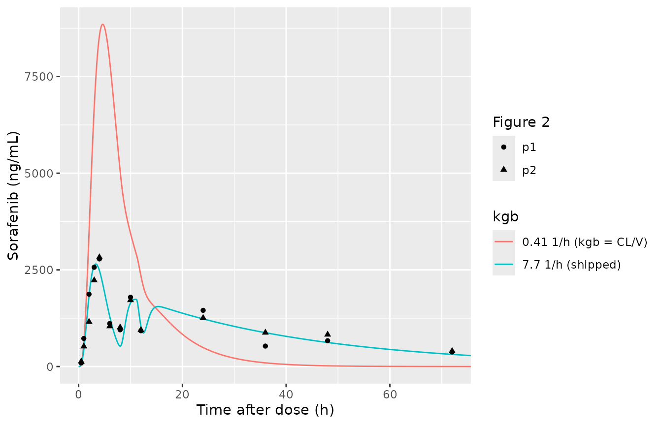
Typical Nexavar 200 mg profile with the shipped kgb (7.7 1/h) and with the Jain 2011 reading kgb = CL/V (0.41 1/h), against the digitised Figure 2 means (points: period 1 and period 2).
Mass balance
The transit input carries the dose and the bioavailability, so a long
typical-value solve must recover
AUC = F * Dose / ((1 - Fent) * CL) exactly. This also
guards against the transit input silently delivering no drug.
ev_mb <- rxode2::et(amt = 200, cmt = "depot") |>
  rxode2::et(seq(0, 2000, by = 0.25)) |>
  as.data.frame() |>
  mutate(FORM_SORAFENIB_SYO1644 = 0, OCC = 1)
s_mb <- rxode2::rxSolve(mod_typical, ev_mb, returnType = "data.frame")
#> ℹ omega/sigma items treated as zero: 'etalka', 'etalcl', 'etalvc', 'etaiov_cl_1', 'etaiov_cl_2'
auc_num <- sum(diff(s_mb$time) * (head(s_mb$Cc, -1) + tail(s_mb$Cc, -1)) / 2)
auc_expected <- 200 / ((1 - mod$theta[["fent"]]) * exp(mod$theta[["lcl"]])) * 1000
c(numerical = auc_num, expected = auc_expected)
#> numerical  expected
#>  76509.73  76509.63
stopifnot(abs(auc_num / auc_expected - 1) < 0.005)
Virtual cohort
Each arm has 200 virtual subjects. Every subject receives the arm’s
dose at time 0 (period 1, OCC = 1) and again at 336 h
(period 2, OCC = 2), and is sampled at the study’s nominal
times after each dose plus a dense grid for plotting. The model has no
demographic covariates, so only the formulation indicator and the
occasion vary.
arms <- tibble::tribble(
  ~treatment,           ~amt, ~FORM_SORAFENIB_SYO1644,
  "SYO-1644 100 mg",    100,  1,
  "SYO-1644 150 mg",    150,  1,
  "SYO-1644 200 mg",    200,  1,
  "Nexavar 200 mg",     200,  0
)
n_per_arm <- 200
t_period2 <- 336
nominal <- c(0, 0.5, 1, 2, 3, 4, 6, 8, 10, 12, 24, 36, 48, 72, 96, 120, 168)
obs_times <- sort(unique(c(nominal, seq(0, 24, by = 0.5), seq(24, 168, by = 4))))

make_arm <- function(i) {
  a <- arms[i, ]
  ids <- (i - 1) * n_per_arm + seq_len(n_per_arm)
  dose <- tidyr::expand_grid(id = ids, period = 1:2) |>
    mutate(time = (period - 1) * t_period2, evid = 1, amt = a$amt)
  obs <- tidyr::expand_grid(id = ids, period = 1:2, tad_nom = obs_times) |>
    mutate(time = (period - 1) * t_period2 + tad_nom, evid = 0, amt = 0)
  bind_rows(dose, obs) |>
    mutate(
      cmt = "depot",
      treatment = a$treatment,
      FORM_SORAFENIB_SYO1644 = a$FORM_SORAFENIB_SYO1644,
      OCC = period
    ) |>
    arrange(id, time, desc(evid)) |>
    select(id, time, evid, amt, cmt, period, treatment, FORM_SORAFENIB_SYO1644, OCC)
}
events <- bind_rows(lapply(seq_len(nrow(arms)), make_arm))
stopifnot(!anyDuplicated(unique(events[, c("id", "time", "evid")])))
Simulation
rxode2::rxSetSeed(2021)
sim <- rxode2::rxSolve(mod, events = events, keep = c("treatment", "period")) |>
  as.data.frame() |>
  mutate(
    tad_h = time - (period - 1) * t_period2,
    treatment = factor(treatment, levels = arms$treatment)
  )
# A silently zero transit input would leave every concentration at 0.
stopifnot(max(sim$Cc) > 1000)
Replicate published figures
sim |>
  filter(period == 1) |>
  group_by(treatment, tad_h) |>
  summarise(Cc = mean(Cc), .groups = "drop") |>
  ggplot(aes(tad_h, Cc, colour = treatment)) +
  geom_line() +
  geom_point(
    data = fig2_nexavar |> pivot_longer(c(p1, p2), names_to = "period", values_to = "obs"),
    aes(time, obs), inherit.aes = FALSE, colour = "black"
  ) +
  labs(x = "Time after dose (h)", y = "Sorafenib (ng/mL)", colour = NULL)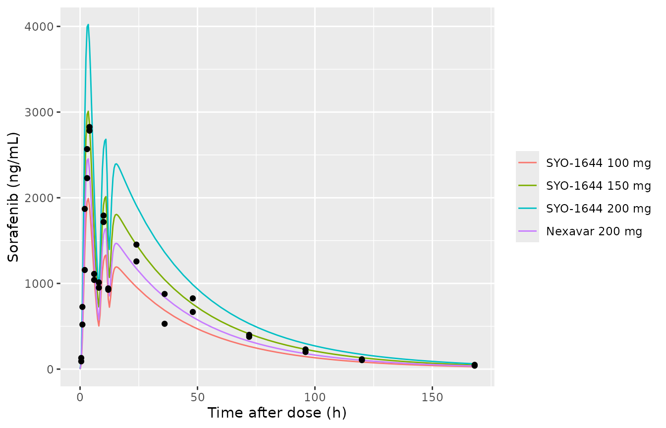
Replicates Figure 2 of Huh 2021: arithmetic mean sorafenib concentration by treatment (period 1, model prediction without residual error); points are the digitised Nexavar 200 mg means of periods 1 and 2.
sim |>
  group_by(treatment, tad_h) |>
  summarise(
    Q05 = quantile(sim, 0.05), Q50 = quantile(sim, 0.50), Q95 = quantile(sim, 0.95),
    .groups = "drop"
  ) |>
  ggplot(aes(tad_h, Q50)) +
  geom_ribbon(aes(ymin = Q05, ymax = Q95), alpha = 0.25, fill = "steelblue") +
  geom_line(colour = "firebrick") +
  facet_wrap(~treatment) +
  coord_cartesian(ylim = c(0, 10000)) +
  labs(x = "Time after dose (h)", y = "Plasma sorafenib (ng/mL)")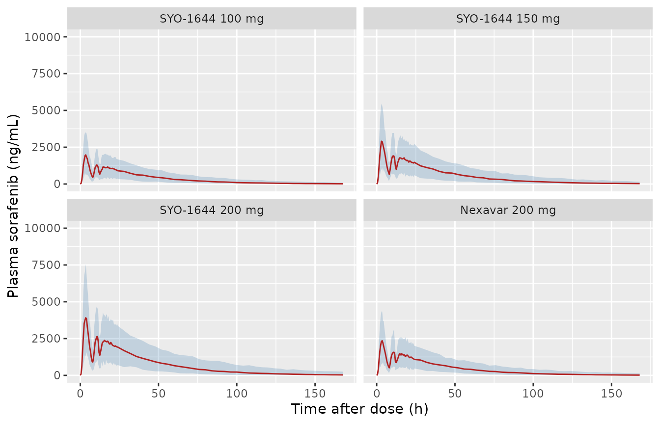
Replicates Figure 4 of Huh 2021: simulated 5th, 50th and 95th percentiles by treatment (both periods pooled, residual error included).
PKNCA validation
The NCA uses the study’s nominal sampling times and the simulated
observations with residual error (sim), which is how Table
1 was derived from measured data. Values below the 5 ng/mL lower limit
of quantification (Methods 2.3), including the rare negative draws of
the proportional error, are excluded.
# Pre-dose records are 0; post-dose records below the LLOQ become NA.
sim_nca <- sim |>
  mutate(Cc = dplyr::case_when(
    !(tad_h %in% nominal) ~ NA_real_,
    tad_h == 0 ~ 0,
    sim < 5 ~ NA_real_,
    TRUE ~ sim
  )) |>
  filter(!is.na(Cc)) |>
  select(id, period, treatment, time = tad_h, Cc)
stopifnot(all(tapply(sim_nca$time == 0, paste(sim_nca$id, sim_nca$period), any)))

dose_nca <- events |>
  filter(evid == 1) |>
  mutate(time = 0, treatment = factor(treatment, levels = arms$treatment)) |>
  select(id, period, treatment, time, amt)

conc_obj <- PKNCA::PKNCAconc(sim_nca, Cc ~ time | treatment + period + id)
dose_obj <- PKNCA::PKNCAdose(dose_nca, amt ~ time | treatment + period + id)
intervals <- data.frame(
  start = 0, end = 168,
  cmax = TRUE, tmax = TRUE, auclast = TRUE, half.life = TRUE
)
nca_res <- PKNCA::pk.nca(PKNCA::PKNCAdata(conc_obj, dose_obj, intervals = intervals))
Comparison against published NCA
Table 1 reports means for Cmax, AUClast and t1/2 and the median for Tmax, so the simulated results are summarised the same way before comparison.
nca_long <- as.data.frame(nca_res$result) |>
  filter(PPTESTCD %in% c("cmax", "tmax", "auclast", "half.life"))
sim_summary <- nca_long |>
  group_by(treatment, PPTESTCD) |>
  summarise(
    PPORRES = if (PPTESTCD[1] == "tmax") median(PPORRES, na.rm = TRUE) else mean(PPORRES, na.rm = TRUE),
    .groups = "drop"
  ) |>
  mutate(treatment = as.character(treatment))

published <- tibble::tribble(
  ~treatment,        ~cmax,  ~auclast, ~tmax, ~half.life,
  "SYO-1644 100 mg", 3015.8, 55676.6,  4.0,   20.9,
  "SYO-1644 150 mg", 4899.4, 89241.2,  4.0,   24.7,
  "SYO-1644 200 mg", 5037.5, 105312.9, 4.0,   24.4,
  "Nexavar 200 mg",  2953.4, 73730.1,  4.0,   22.2
)

cmp <- nlmixr2lib::ncaComparisonTable(
  simulated = sim_summary,
  reference = published,
  by = "treatment",
  units = c(cmax = "ng/mL", auclast = "h*ng/mL", tmax = "h", half.life = "h"),
  tolerance_pct = 20
)
knitr::kable(cmp, caption = "Simulated vs. published NCA (Huh 2021 Table 1). * differs from the published value by more than 20%.")| NCA parameter | treatment | Reference | Simulated | % diff |
|---|---|---|---|---|
| Cmax (ng/mL) | SYO-1644 100 mg | 3020 | 2450 | -18.9% |
| Cmax (ng/mL) | SYO-1644 150 mg | 4900 | 3710 | -24.2%* |
| Cmax (ng/mL) | SYO-1644 200 mg | 5040 | 4940 | -1.9% |
| Cmax (ng/mL) | Nexavar 200 mg | 2950 | 2940 | -0.5% |
| Tmax (h) | SYO-1644 100 mg | 4 | 4 | +0.0% |
| Tmax (h) | SYO-1644 150 mg | 4 | 3 | -25.0%* |
| Tmax (h) | SYO-1644 200 mg | 4 | 4 | +0.0% |
| Tmax (h) | Nexavar 200 mg | 4 | 3 | -25.0%* |
| AUClast (h*ng/mL) | SYO-1644 100 mg | 55700 | 57700 | +3.7% |
| AUClast (h*ng/mL) | SYO-1644 150 mg | 89200 | 89300 | +0.1% |
| AUClast (h*ng/mL) | SYO-1644 200 mg | 105000 | 118000 | +11.8% |
| AUClast (h*ng/mL) | Nexavar 200 mg | 73700 | 69500 | -5.8% |
| t½ (h) | SYO-1644 100 mg | 20.9 | 25.7 | +22.8%* |
| t½ (h) | SYO-1644 150 mg | 24.7 | 25.9 | +4.9% |
| t½ (h) | SYO-1644 200 mg | 24.4 | 26.1 | +7.1% |
| t½ (h) | Nexavar 200 mg | 22.2 | 26.5 | +19.4% |
AUClast agrees within 12% in every arm and Nexavar Cmax within 1%. The flagged rows are SYO-1644 150 mg Cmax (-24%; Table 1’s 150 mg arm has the largest Cmax CV, 51.5%, from 7 subjects), the median Tmax of 3 h against the observed 4 h in two arms (the simulated individual peaks split between the 3 h and 4 h samples), and the 100 mg half-life. The simulated terminal half-lives of about 26 h sit slightly above the observed 21-25 h range; the terminal phase is set by CL, V, Fent and the unreported kgb together.
pct <- sim_summary |>
  inner_join(
    published |> pivot_longer(-treatment, names_to = "PPTESTCD", values_to = "ref"),
    by = c("treatment", "PPTESTCD")
  ) |>
  mutate(pct_diff = 100 * (PPORRES - ref) / ref)
auc_pct <- pct$pct_diff[pct$PPTESTCD == "auclast"]
cmax_pct <- pct$pct_diff[pct$PPTESTCD == "cmax"]
# Structural: a wrong clearance, Fent, F or unit moves AUC by tens of percent
# in every arm at once. Centre and envelope, not extremes.
stopifnot(
  abs(median(auc_pct)) < 20,
  max(abs(auc_pct)) < 35,
  abs(median(cmax_pct)) < 25
)
Equivalent dose and intra-subject variability
Because the model is linear in dose, the SYO-1644 dose with the same
typical exposure as Nexavar 200 mg is
200 / 1.62 = 123.5 mg, inside the 120-125 mg range that the
paper’s 500-trial bioequivalence simulations identified (Results 3.4,
Table S2).
eq_dose <- 200 / exp(mod$theta[["e_form_syo1644_fdepot"]])
eq_dose
#> [1] 123.4568
stopifnot(eq_dose >= 120, eq_dose <= 125)
A 2 x 2 crossover of Nexavar 200 mg (period 1) against SYO-1644 120 mg or 125 mg (period 2), 200 subjects per comparison, gives the geometric mean ratios and the intra-subject CVs. Within a subject, the two periods differ only through the inter-occasion variability on CL and the residual error, so the intra-subject CV is a check on those two variance terms. Table S3 reports a median intra-subject CV of 22.0% for Cmax and 15.7% for AUClast in the paper’s simulated trials.
make_crossover <- function(syo_dose, id_offset) {
  ids <- id_offset + seq_len(n_per_arm)
  per <- tibble::tibble(
    period = 1:2, amt = c(200, syo_dose), FORM_SORAFENIB_SYO1644 = c(0, 1)
  )
  dose <- tidyr::expand_grid(id = ids, period = 1:2) |>
    left_join(per, by = "period") |>
    mutate(time = (period - 1) * t_period2, evid = 1)
  obs <- tidyr::expand_grid(id = ids, period = 1:2, tad_nom = nominal) |>
    left_join(per |> mutate(amt = 0), by = "period") |>
    mutate(time = (period - 1) * t_period2 + tad_nom, evid = 0)
  bind_rows(dose, obs) |>
    mutate(cmt = "depot", OCC = period, comparison = paste0("SYO-1644 ", syo_dose, " mg vs Nexavar 200 mg")) |>
    arrange(id, time, desc(evid)) |>
    select(id, time, evid, amt, cmt, period, comparison, FORM_SORAFENIB_SYO1644, OCC)
}
ev_be <- bind_rows(make_crossover(120, 10000L), make_crossover(125, 20000L))
stopifnot(!anyDuplicated(unique(ev_be[, c("id", "time", "evid")])))

sim_be <- rxode2::rxSolve(mod, events = ev_be, keep = c("comparison", "period")) |>
  as.data.frame() |>
  mutate(tad_h = time - (period - 1) * t_period2) |>
  filter(tad_h %in% nominal)

# Linear-up/log-down AUClast as in Methods 2.4, values below the LLOQ dropped.
auc_lin_log <- function(t, c) {
  ok <- !is.na(c)
  t <- t[ok]; c <- c[ok]
  dt <- diff(t); c1 <- head(c, -1); c2 <- tail(c, -1)
  seg <- ifelse(c2 < c1 & c2 > 0, dt * (c1 - c2) / log(c1 / c2), dt * (c1 + c2) / 2)
  sum(seg)
}
be_ind <- sim_be |>
  mutate(Cobs = ifelse(tad_h == 0, 0, ifelse(sim < 5, NA_real_, sim))) |>
  group_by(comparison, id, period) |>
  summarise(cmax = max(Cobs, na.rm = TRUE), auclast = auc_lin_log(tad_h, Cobs), .groups = "drop")

be <- be_ind |>
  pivot_longer(c(cmax, auclast), names_to = "parameter") |>
  pivot_wider(names_from = period, values_from = value, names_prefix = "p") |>
  mutate(d = log(p2) - log(p1)) |>
  group_by(comparison, parameter) |>
  summarise(
    n = n(),
    gmr = exp(mean(d)),
    lo90 = exp(mean(d) - qt(0.95, n - 1) * sd(d) / sqrt(n)),
    hi90 = exp(mean(d) + qt(0.95, n - 1) * sd(d) / sqrt(n)),
    cv_intra = 100 * sqrt(exp(var(d) / 2) - 1),
    .groups = "drop"
  )
be |>
  mutate(across(c(gmr, lo90, hi90), ~ round(.x, 3)), cv_intra = round(cv_intra, 1)) |>
  dplyr::rename(
    "Comparison" = comparison, "Parameter" = parameter, "N" = n, "GMR" = gmr,
    "90% CI lower" = lo90, "90% CI upper" = hi90, "Intra-subject CV (%)" = cv_intra
  ) |>
knitr::kable(caption = "Simulated 2 x 2 crossover: geometric mean ratio (SYO-1644 / Nexavar 200 mg) with 90% CI and intra-subject CV.")| Comparison | Parameter | N | GMR | 90% CI lower | 90% CI upper | Intra-subject CV (%) |
|---|---|---|---|---|---|---|
| SYO-1644 120 mg vs Nexavar 200 mg | auclast | 200 | 0.978 | 0.953 | 1.003 | 15.5 |
| SYO-1644 120 mg vs Nexavar 200 mg | cmax | 200 | 0.953 | 0.920 | 0.988 | 22.0 |
| SYO-1644 125 mg vs Nexavar 200 mg | auclast | 200 | 1.010 | 0.983 | 1.038 | 16.5 |
| SYO-1644 125 mg vs Nexavar 200 mg | cmax | 200 | 0.997 | 0.963 | 1.032 | 21.3 |
The simulated intra-subject CVs reproduce Table S3 (22.0% for Cmax and 15.7% for AUClast) closely, which supports the inter-occasion and residual-error magnitudes as transcribed, and both candidate doses give geometric mean ratios near 1 with 90% confidence intervals well inside 0.80-1.25.
# Both candidate doses sit inside the 0.80-1.25 bioequivalence limits.
stopifnot(all(be$gmr > 0.85 & be$gmr < 1.18))
# Table S3: median intra-subject CV 22.0% (Cmax) and 15.7% (AUClast). The
# bounds admit the spread of a 200-subject estimate while still failing on a
# missing or mis-scaled IOV or residual-error term.
cv_cmax <- mean(be$cv_intra[be$parameter == "cmax"])
cv_auc <- mean(be$cv_intra[be$parameter == "auclast"])
c(cmax = cv_cmax, auclast = cv_auc)
#>     cmax  auclast
#> 21.68103 16.02065
stopifnot(abs(cv_cmax - 22.0) < 8, abs(cv_auc - 15.7) < 7)
Assumptions and deviations
-
kgbback-solved by the maintainers. The central-to-gallbladder rate constant drawn in Figure 3 is not reported anywhere in the paper or its supplement. Jain 2011’s assumptionkgb = CL/V(0.41 1/h) does not reproduce Figure 2, sokgbwas fitted at 7.7 1/h to the digitised Figure 2 Nexavar 200 mg mean profile with all other parameters at their Table 2 values (population-mean fit; a typical-value fit gives 8.1-8.9 1/h). The value should be replaced if the authors publish it. The productFent * kgbat this value is about 1.66 1/h, close to the estimated ka of 1.6 1/h; nothing in the paper says whether that is more than a coincidence. - Residual error is proportional only. Methods 2.5 describes a combined proportional and additive error model, but Table 2 reports only the proportional term (37.6%). No additive term is included.
-
Transit chain convention. The model uses the Savic
closed-form transit input with
ktr = (NN + 1) / MTTand a separately estimatedkaout of the absorption compartment, which is the parameterisation that a non-integerNNimplies. Figure 3 labels every arrow of the transit chainka, which is read as a drawing convention carried over from Jain 2011’s diagram, where all the chain’s rate constants were equal. -
Gallbladder release target. Figure 3 draws the
gallbladder output entering the last transit compartment before central,
and the text calls it “the absorption compartment”; it is encoded as an
input to the absorption compartment that empties into central at
ka. -
Inter-occasion variability. Two occasions, one per
study period, share one variance (the
$OMEGA BLOCK(1) SAMEidiom described in Methods 2.5). -
Hill switch reset. Equation 3 is implemented as
written: the sigmoid is centred on Tgb1 until
Tgb1 + 3h after the dose and on Tgb2 from then on, so the gallbladder empties continuously atkEhcafter about 12 h. - NCA summaries. Table 1 reports arithmetic means (median for Tmax) of 7-8 completers per arm; the simulation uses 200 subjects per arm, nominal times and the 5 ng/mL LLOQ. The popPK relative bioavailability of 1.62 exceeds the NCA AUClast ratio (1.51, Discussion), so the simulated SYO-1644 AUCs sit above Table 1 by more than the Nexavar AUC does.
- No correction notice for the article was found in Europe PMC or in the Crossref update metadata for its DOI (checked 2026-10-16).