Entinostat + nivolumab + ipilimumab HER2-negative breast cancer QSP (Wang 2020)
Source:vignettes/articles/Wang_2020_entinostat_nivolumab_ipilimumab_qsp.Rmd
Wang_2020_entinostat_nivolumab_ipilimumab_qsp.Rmd
# Build once and reuse: this is a 120-state model, and every extra build costs
# several seconds.
mod <- rxode2::rxode2(readModelDb("Wang_2020_entinostat_nivolumab_ipilimumab_qsp"))
Model and source
- Citation: Wang H, Sove RJ, Jafarnejad M, Rahmeh S, Jaffee EM, Stearns V, Torres ETR, Connolly RM, Popel AS. Conducting a Virtual Clinical Trial in HER2-Negative Breast Cancer Using a Quantitative Systems Pharmacology Model With an Epigenetic Modulator and Immune Checkpoint Inhibitors. Front Bioeng Biotechnol. 2020;8:141. doi:10.3389/fbioe.2020.00141.
- Article: https://doi.org/10.3389/fbioe.2020.00141
This is a deterministic quantitative systems pharmacology (QSP) model
of HER2-negative breast cancer under immune checkpoint blockade with
nivolumab (anti-PD-1) and ipilimumab (anti-CTLA-4), combined with the
class I histone deacetylase inhibitor entinostat. It is a member of the
Popel-laboratory immuno-oncology QSP family (see also
Anbari_2023_atezolizumab_cibisatamab_qsp,
Ippolito_2024_pacmilimab_qsp and
Wang_2024_evorpacept_qsp).
The authors built it in SimBiology and deposited the model with the
article: an SBML export (Immune_Oncology_Model.xml) plus a
workbook of the full model listing – compartments (Supplementary Table
S1), parameters (S2), reactions and rate laws (S3), algebraic rules
(S4), species and initial amounts (S5), the single event (S6) and the
MDSC-module parameters (S7). The packaged model is a translation of the
SBML deposit, with every value checked against the printed tables (the
eight places where they differ are listed under Assumptions and
deviations).
The paper’s own contributions over the earlier platform are:
- an entinostat PK/PD module (Figure 2): a fraction
Fof each oral dose is absorbed through a zero-order buccal route overD0, the rest through a lagged first-order gastrointestinal route; distribution to the peripheral, tumour and lymph-node compartments; linear plus Michaelis-Menten clearance; inhibition of cancer-cell proliferation and of CCL2, nitric-oxide and arginase-I production; - an MDSC module: CCL2-driven MDSC recruitment, arginase-I and nitric-oxide inhibition of effector T cell (Teff) killing, and arginase-I driven Treg expansion;
- anti-CTLA-4 ADCC: ipilimumab-bound CTLA-4 on Tregs drives Treg depletion.
There are no etas and no residual-error model. The authors did not fit inter-individual variability: they generated 1500 virtual patients by Latin hypercube sampling of the parameter ranges printed in brackets in Table S2, of which 1196 reached a preselected pre-treatment tumour size. The model is packaged as a typical-individual mechanism model.
How the translation works
SimBiology converts units implicitly; rxode2 does not. Every
parameter value was therefore converted to one consistent unit system –
amounts in counts (the export itself defines 1 cell = 1 molecule =
1/Avogadro mol), volumes in litres, areas in dm^2, time in days – and
every one of the 154 rate laws, 21 rules and 18 initial assignments was
checked by a dimensional-analysis pass that requires each rate to reduce
to amount/time. The ODE states hold amounts
(q_<compartment>_<species>); the
x_<compartment>_<species> variables are the
SimBiology species values (concentrations for species that SimBiology
stores as concentrations). Integrating amounts is what SimBiology does
internally and handles the time-varying tumour volume without any
dilution term.
The four drug families (nivolumab, ipilimumab, durvalumab and entinostat, including the two entinostat depots) are held in nmol, so dose records are in nmol. All other states (cells, surface molecules, cytokines, antigens) are held in counts.
Model outputs: tumour_diameter (cm, from the total
tumour volume assuming a sphere), Cc_nivolumab,
Cc_ipilimumab, Cc_entinostat (central
concentrations, nmol/L) and the tumour-infiltrating cell densities
teff_density, treg_density,
mdsc_density (cells per mL of tumour).
Dosing
- Nivolumab, ipilimumab (and durvalumab): IV doses, in nmol, into
q_V_C_nivo,q_V_C_ipi(q_V_C_durv). - Entinostat: give the same nmol amount twice at each
dosing time – once into
q_V_C_ENT_Buccalwithrate = -2(the model supplies the zero-order durationdurP) and once intoq_V_C_Dose2. The model splits the dose withf(q_V_C_ENT_Buccal) <- F_ENT_buccalandf(q_V_C_Dose2) <- 1 - F_ENT_buccal, and applies the gastrointestinal lagalag(q_V_C_Dose2) <- lagP.
The pre-treatment phase
As in the paper, a simulation starts from a single cancer cell
(q_V_T_C1(0) = 1) with no T cells anywhere, and the tumour
is grown until it reaches the chosen pre-treatment diameter; therapy
then starts. Because the pre-treatment phase contains no doses, it is
enough to run the untreated model once to find the time at which the
tumour reaches that diameter, and then to schedule the first dose at
that time.
Population
The virtual population is described in the Methods (“In silico
Virtual Clinical Trial”) and Results of Wang 2020. It mirrors the
clinical trial NCT02453620 (nivolumab plus entinostat, with or without
ipilimumab, in 26 patients with HER2-negative breast cancer). Baseline
parameter values were estimated from triple-negative breast cancer
(TNBC) data and the sampling ranges from TNBC plus
oestrogen-receptor-positive/HER2-negative data. 1196 of 1500 sampled
parameter sets reached a pre-treatment tumour diameter drawn from
1.1-4.5 cm (Table S2, initial_tumour_diameter), and each
regimen was then simulated for 400 days. The packaged model carries the
reference (baseline) value of every parameter.
Source trace
| Model element | Source |
|---|---|
9 compartments and capacities (vol_*) |
Supplementary Table S1; SBML listOfCompartments
|
196 ini() values: 8 compartment capacities, 187 model
parameters and F_ENT_buccal
|
Supplementary Table S2 (value, unit and description in each line’s comment); MDSC module also Table S7 |
Reaction rates v1-v154
|
Supplementary Table S3 rows 1-154 (numbered identically; rate laws
from the SBML kineticLaw elements, which carry the
compartment-volume factors SimBiology adds to concentration-per-time
rates) |
Tumour volume vol_V_T and the other repeated-assignment
rules |
Supplementary Table S4 |
| Species, locations and initial amounts; synapse and CTLA-4 initial assignments | Supplementary Table S5 and Table S4 (initialAssignment
rows) |
Cancer-cell elimination below 0.9 cells (c1_alive) |
Supplementary Table S6 |
Entinostat absorption scheme (buccal zero-order over
durP, lagged gastrointestinal first-order) |
Figure 2A and Methods “Pharmacokinetics and Pharmacodynamics (PK/PD)
of Entinostat”; Table S2 lagP, durP,
k_dose2, k_a1_ENT, k_a2_ENT
|
F_ENT_buccal = 0.324 |
Not printed; back-solved by the maintainers from the Results text (Cmax 15.4 ng/mL after 2 mg/m^2, body surface area 1.7 m^2) – see below |
| Regimens (nivolumab 3 mg/kg q2w; entinostat 5 mg weekly; ipilimumab 1 mg/kg q6w x 4) | Results, “Efficacy of Anti-PD-1 Monotherapy…” and “Model-Predicted Anti-tumoral Effect in Triple Combination Therapy” |
| Entinostat PK targets (Cmax 15.4/30.8/46.3 ng/mL, AUC 105.5/211.0/316.8 ng h/mL, tmax 0.5 h) | Results, “Prediction of Entinostat Concentration in Tumor”; Figure 2B |
Simulation set-up
# Dosing conversions for the vignette (not model parameters): body weight for
# the mg/kg antibody doses and molecular weights for mg -> nmol.
wt_kg <- 70
mw <- c(nivolumab = 146000, ipilimumab = 148000, entinostat = 376.41) # g/mol
nivo_nmol <- 3 * wt_kg / mw[["nivolumab"]] * 1e6
ipi_nmol <- 1 * wt_kg / mw[["ipilimumab"]] * 1e6
ent_nmol <- 5 / mw[["entinostat"]] * 1e6

# method = "cvode", the SUNDIALS BDF integrator. With lsoda these solves sit on
# a numerical knife-edge: perturbing k_cln_ENT and F_ENT_buccal by one part in
# 1e12 made about 1.5% of the entinostat profiles fail with repeated corrector
# convergence failures, so the same code could fail on one machine and pass on
# another. Tightening the tolerances made it worse. cvode solved all 1200 such
# perturbed entinostat solves, and all 1800 solves of this article's full set
# with every non-integer parameter perturbed the same way, at a similar total
# cost. At the default tolerances it reproduces an rtol = 1e-8 solve to within
# about 5e-4 (relative) in every reported quantity. The default liblsoda
# solver took ~55 s on the 4 mg/m^2 entinostat profile.
SOLVE <- function(ev, params = NULL) {
  rxode2::rxSolve(mod, ev, params = params, method = "cvode", maxsteps = 1e6, returnType = "data.frame")
}

# entinostat dose records: the same amount into both depots
ent_doses <- function(ev, time, amt, ii = 0, addl = 0) {
  ev |>
    rxode2::et(time = time, amt = amt, cmt = "q_V_C_ENT_Buccal", rate = -2, ii = ii, addl = addl) |>
    rxode2::et(time = time, amt = amt, cmt = "q_V_C_Dose2", ii = ii, addl = addl)
}
Replicating Figure 2B: entinostat pharmacokinetics
Single oral doses of 2, 4 and 6 mg/m^2 with a body surface area of 1.7 m^2 (as in the Results). Entinostat kinetics do not depend on the tumour, so the dose is given at time zero.
ent_grid <- sort(unique(c(seq(0, 2, by = 0.02), seq(2, 400, by = 0.5)))) / 24 # days
ent_levels <- c(2, 4, 6) # mg/m^2
ent_pk <- bind_rows(lapply(ent_levels, function(lv) {
  amt <- lv * 1.7 / mw[["entinostat"]] * 1e6
  ev <- ent_doses(rxode2::et(ent_grid), time = 0, amt = amt)
  s <- SOLVE(ev)
  data.frame(
    treatment = paste(lv, "mg/m^2"),
    time_h = s$time * 24,
    conc = s$Cc_entinostat * mw[["entinostat"]] / 1000 # nmol/L -> ng/mL
  )
}))
ent_pk$id <- as.integer(factor(ent_pk$treatment, levels = paste(ent_levels, "mg/m^2")))
ggplot(filter(ent_pk, time_h >= 0.1), aes(time_h, conc, colour = treatment)) +
  geom_line(linewidth = 0.8) +
  scale_x_log10() +
  labs(x = "Time (h)", y = "Entinostat plasma concentration (ng/mL)", colour = NULL) +
  theme_bw()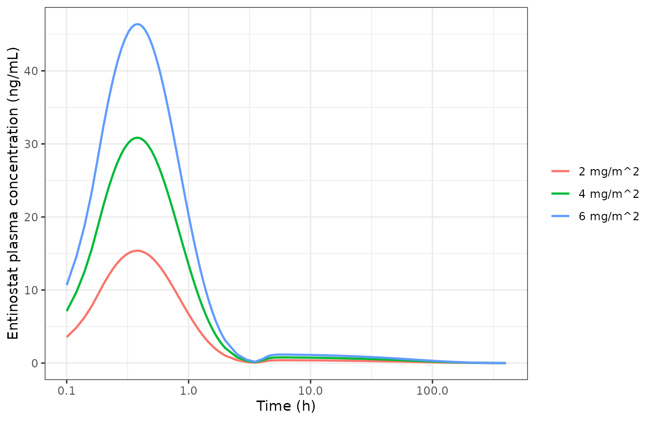
Replicates Figure 2B of Wang 2020: simulated entinostat plasma concentration after single oral doses of 2, 4 and 6 mg/m^2 (log time axis).
Non-compartmental analysis
conc_df <- ent_pk |> select(id, treatment, time = time_h, conc)
dose_df <- conc_df |>
  distinct(id, treatment) |>
  mutate(time = 0, dose = c(2, 4, 6)[id] * 1.7)
o_conc <- PKNCA::PKNCAconc(conc_df, conc ~ time | treatment + id)
o_dose <- PKNCA::PKNCAdose(dose_df, dose ~ time | treatment + id)
intervals <- data.frame(start = 0, end = 400, cmax = TRUE, tmax = TRUE, auclast = TRUE)
nca <- PKNCA::pk.nca(PKNCA::PKNCAdata(o_conc, o_dose, intervals = intervals))

reference <- data.frame(
  treatment = paste(ent_levels, "mg/m^2"),
  cmax = c(15.4, 30.8, 46.3),
  tmax = c(0.5, 0.5, 0.5),
  auclast = c(105.5, 211.0, 316.8)
)
tbl <- nlmixr2lib::ncaComparisonTable(
  nca, reference,
  by = "treatment",
  units = c(cmax = "ng/mL", tmax = "h", auclast = "ng*h/mL")
)
knitr::kable(tbl, caption = "Entinostat NCA: Results text of Wang 2020 (Reference) vs the packaged model (Simulated), AUC over 0-400 h (the absorption tail of the gastrointestinal route is complete by then).")| NCA parameter | treatment | Reference | Simulated | % diff |
|---|---|---|---|---|
| Cmax (ng/mL) | 2 mg/m^2 | 15.4 | 15.4 | -0.1% |
| Cmax (ng/mL) | 4 mg/m^2 | 30.8 | 30.9 | +0.2% |
| Cmax (ng/mL) | 6 mg/m^2 | 46.3 | 46.4 | +0.2% |
| Tmax (h) | 2 mg/m^2 | 0.5 | 0.38 | -24.0%* |
| Tmax (h) | 4 mg/m^2 | 0.5 | 0.38 | -24.0%* |
| Tmax (h) | 6 mg/m^2 | 0.5 | 0.38 | -24.0%* |
| AUClast (ng*h/mL) | 2 mg/m^2 | 106 | 42.9 | -59.3%* |
| AUClast (ng*h/mL) | 4 mg/m^2 | 211 | 85.9 | -59.3%* |
| AUClast (ng*h/mL) | 6 mg/m^2 | 317 | 129 | -59.3%* |
nca_res <- as.data.frame(nca$result)
cmax_sim <- nca_res |> filter(PPTESTCD == "cmax") |> arrange(treatment) |> pull(PPORRES)
auc_sim <- nca_res |> filter(PPTESTCD == "auclast") |> arrange(treatment) |> pull(PPORRES)
stopifnot(
  # Cmax is the quantity F_ENT_buccal was back-solved to: it must reproduce
  # 15.4 / 30.8 / 46.3 ng/mL (dose-proportional) to within 1 percent.
  all(abs(cmax_sim / c(15.4, 30.8, 46.3) - 1) < 0.01),
  # Entinostat is linear at these doses (C << Kc_ENT): AUC scales with dose.
  all(abs(auc_sim / auc_sim[1] / c(1, 2, 3) - 1) < 0.01)
)
F_ENT_buccal is not printed anywhere in the article or
supplement (the authors’ dosing scripts are available only on request).
Because the plasma Cmax is set almost entirely by the buccal fraction,
it was back-solved from the 2 mg/m^2 Cmax of 15.4 ng/mL; the 4 and 6
mg/m^2 values then follow by dose proportionality.
The published AUC is not reproduced. With the
printed parameters the simulated AUC is about 40 percent of the
published 105.5 / 211.0 / 316.8 ng h/mL (starred rows), and the
gastrointestinal “hump” of Figure 2B around 10 h is about three times
lower than drawn. The simulated tmax is 0.38 h against the 0.5 h in the
text (also starred); the peak falls between the 0.1-h points plotted in
Figure 2B, and the reading below moves it to 0.56 h. No value of
F_ENT_buccal can fix this: over the dosing interval
essentially the whole dose is absorbed, so the AUC is dose / total
clearance whatever the split, and the printed clearance terms give a
low-concentration clearance of about 79 L/h
(k_cln_ENT / Kc_ENT x V_C = 78 L/h from the
Michaelis-Menten term, plus 0.9 L/h linear), against about 32 L/h
implied by the published AUC.
The published numbers are reproduced jointly if the
Michaelis-Menten capacity k_cln_ENT is 0.4 times its
printed value (4.9e-5 instead of 1.22e-4 mol/L/h, below the printed
range of 6e-5 to 1.22e-4) with the buccal fraction re-solved to 0.184.
That reading is shown below as a sensitivity scenario only. It is
not used in the packaged model: the printed value is
the authors’ deposited parameter, the SBML deposit carries the same
value, and fitting a printed parameter to a reported simulation is not
done in this library.
p_kcln <- mod$iniDf$est[mod$iniDf$name == "k_cln_ENT"]
scen <- bind_rows(lapply(ent_levels, function(lv) {
  amt <- lv * 1.7 / mw[["entinostat"]] * 1e6
  s <- SOLVE(
    ent_doses(rxode2::et(ent_grid), time = 0, amt = amt),
    params = c(k_cln_ENT = 0.4 * p_kcln, F_ENT_buccal = 0.184)
  )
  th <- s$time * 24
  cc <- s$Cc_entinostat * mw[["entinostat"]] / 1000
  data.frame(
    treatment = paste(lv, "mg/m^2"),
    cmax = max(cc),
    tmax = th[which.max(cc)],
    auc_0_400 = sum(diff(th) * (head(cc, -1) + tail(cc, -1)) / 2)
  )
}))
scen |>
  dplyr::rename(
    "Dose" = treatment, "Cmax (ng/mL)" = cmax, "tmax (h)" = tmax,
    "AUC0-400 (ng h/mL)" = auc_0_400
  ) |>
knitr::kable(digits = 2, caption = "Sensitivity scenario (not the packaged model): k_cln_ENT x 0.4 and F_ENT_buccal = 0.184. Published: Cmax 15.4 / 30.8 / 46.3 ng/mL, AUC 105.5 / 211.0 / 316.8 ng h/mL, tmax 0.5 h.")| Dose | Cmax (ng/mL) | tmax (h) | AUC0-400 (ng h/mL) |
|---|---|---|---|
| 2 mg/m^2 | 15.37 | 0.56 | 105.45 |
| 4 mg/m^2 | 30.80 | 0.56 | 211.04 |
| 6 mg/m^2 | 46.29 | 0.56 | 316.77 |
Reference virtual patient
The reference parameter set is grown from a single cancer cell to a pre-treatment diameter of 2.5 cm (inside the 1.1-4.5 cm range of Table S2; the paper does not give a reference value), then treated for 400 days with each of the paper’s regimens.
growth <- SOLVE(rxode2::et(seq(0, 4000, by = 5)))
t_star <- approx(growth$tumour_diameter, growth$time, 2.5)$y
t_star
#> [1] 3300.358
ggplot(growth, aes(time / 365.25, tumour_diameter)) +
  geom_line() +
  geom_hline(yintercept = 2.5, linetype = "dashed") +
  scale_y_log10() +
  labs(x = "Time from the first cancer cell (years)", y = "Tumour diameter (cm)") +
  theme_bw()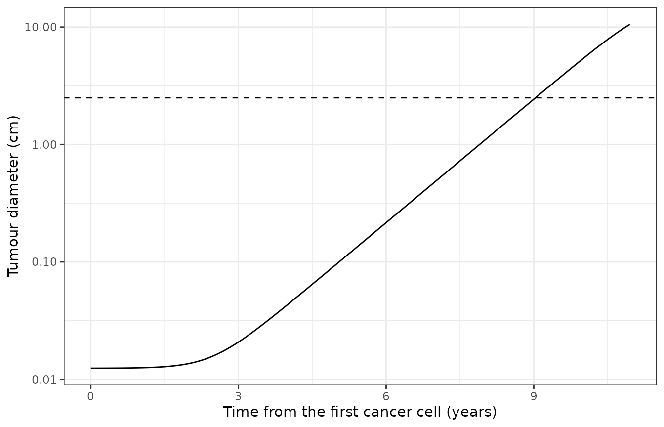
Untreated growth of the reference virtual patient from one cancer cell. The dashed line marks the 2.5 cm pre-treatment diameter.
obs_t <- t_star + seq(0, 400, by = 2)
make_arm <- function(nivo = FALSE, ent = FALSE, ipi = FALSE) {
  ev <- rxode2::et(obs_t)
  if (nivo) ev <- rxode2::et(ev, time = t_star, amt = nivo_nmol, cmt = "q_V_C_nivo", ii = 14, addl = 28)
  if (ent) ev <- ent_doses(ev, time = t_star, amt = ent_nmol, ii = 7, addl = 57)
  if (ipi) ev <- rxode2::et(ev, time = t_star, amt = ipi_nmol, cmt = "q_V_C_ipi", ii = 42, addl = 3)
  ev
}
arm_def <- list(
  "Untreated" = make_arm(),
  "Nivolumab" = make_arm(nivo = TRUE),
  "Nivolumab + entinostat" = make_arm(nivo = TRUE, ent = TRUE),
  "Nivolumab + entinostat + ipilimumab" = make_arm(nivo = TRUE, ent = TRUE, ipi = TRUE)
)
arms <- bind_rows(lapply(names(arm_def), function(a) {
  s <- SOLVE(arm_def[[a]])
  s$arm <- a
  s
}))
arms <- arms |>
  mutate(
    day = time - t_star,
    arm = factor(arm, levels = names(arm_def)),
    pct_change = 100 * (tumour_diameter / 2.5 - 1),
    teff_treg = teff_density / treg_density
  )
ggplot(arms, aes(day, pct_change, colour = arm)) +
  geom_line(linewidth = 0.8) +
  geom_hline(yintercept = c(20, -30), linetype = "dashed") +
  labs(x = "Days from the start of therapy", y = "Change in tumour diameter (%)", colour = NULL) +
  theme_bw() +
  theme(legend.position = "bottom", legend.direction = "vertical")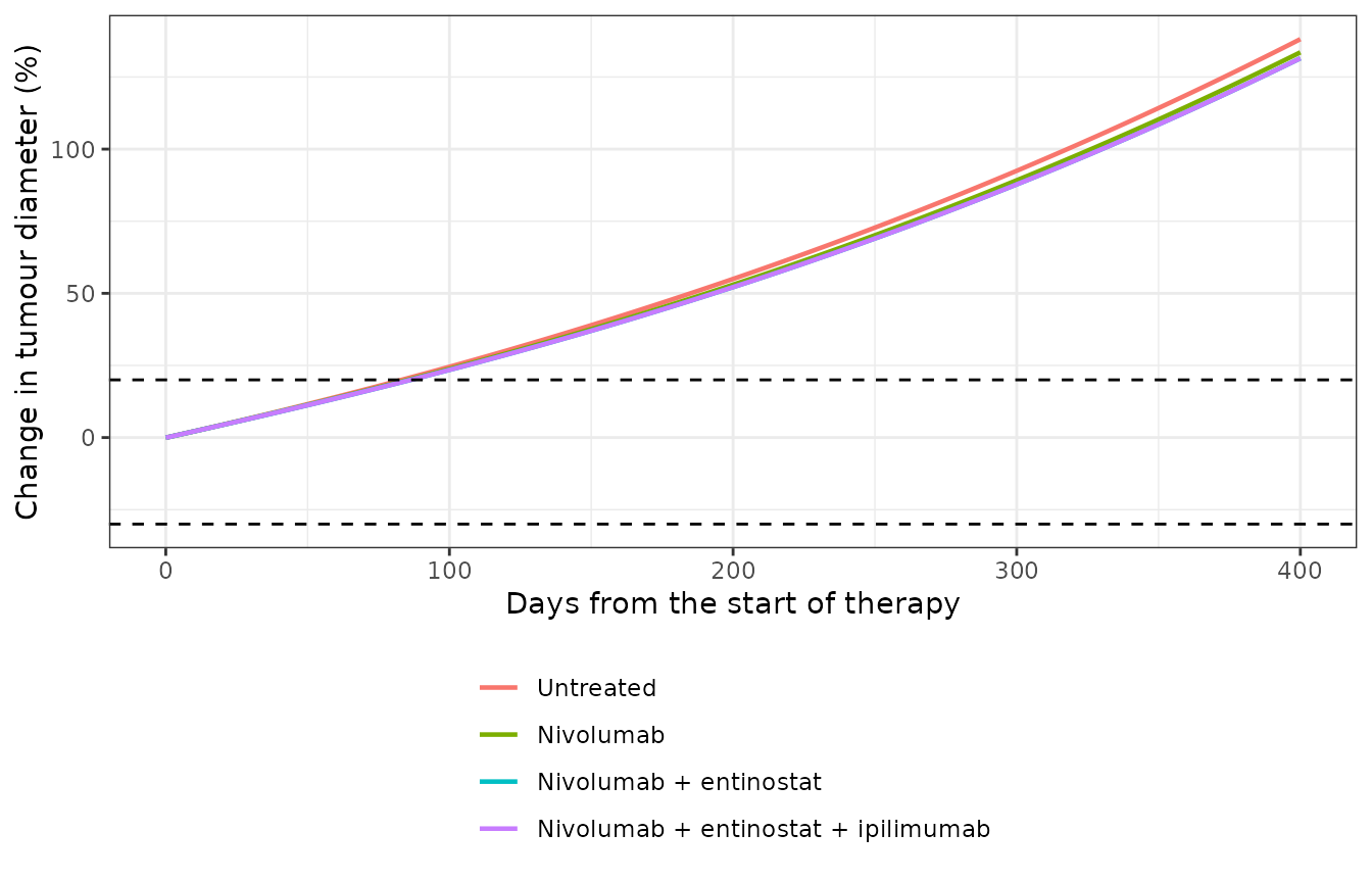
Percentage change in tumour diameter of the reference virtual patient under each regimen (compare the spider plots of Figure 3). Dashed lines: RECIST +20 percent (progression) and -30 percent (partial response).
arm_sum <- arms |>
  group_by(arm) |>
  summarise(
    diam_end = tumour_diameter[which.max(day)],
    pct_end = pct_change[which.max(day)],
    teff_treg_d56 = teff_treg[day == 56],
    teff_d56 = teff_density[day == 56],
    treg_d56 = treg_density[day == 56],
    .groups = "drop"
  )
arm_sum |>
  dplyr::rename(
    "Regimen" = arm, "Diameter at day 400 (cm)" = diam_end,
    "Change at day 400 (%)" = pct_end, "Teff/Treg at day 56" = teff_treg_d56,
    "Teff (cells/mL) at day 56" = teff_d56, "Treg (cells/mL) at day 56" = treg_d56
  ) |>
knitr::kable(digits = 1, caption = "Reference virtual patient: tumour size and tumour-infiltrating T cells by regimen.")| Regimen | Diameter at day 400 (cm) | Change at day 400 (%) | Teff/Treg at day 56 | Teff (cells/mL) at day 56 | Treg (cells/mL) at day 56 |
|---|---|---|---|---|---|
| Untreated | 6.0 | 138.1 | 123.2 | 116447.0 | 945.5 |
| Nivolumab | 5.8 | 133.6 | 204.8 | 193725.5 | 945.7 |
| Nivolumab + entinostat | 5.8 | 131.5 | 205.2 | 194052.4 | 945.8 |
| Nivolumab + entinostat + ipilimumab | 5.8 | 131.5 | 221.7 | 194057.5 | 875.4 |
The reference parameter set is a progressive-disease patient under every regimen, which is the most common outcome in the paper’s virtual cohort (74.8 percent progressive disease under nivolumab; 68.9 percent under nivolumab + entinostat). The mechanistic directions reported in the Results are reproduced:
- nivolumab raises the tumour-infiltrating Teff density and the Teff/Treg ratio (it relieves PD-1 inhibition of Teffs);
- entinostat reduces the MDSC suppression term
H_MDSC_C1(through its inhibition of nitric-oxide and arginase-I production) and slows growth slightly; - adding ipilimumab lowers the Treg density through ADCC and so raises the Teff/Treg ratio further, with little extra change in tumour size (the paper: “While the number of responders remains the same, the mean post-treatment tumor volume is lower than that in the double combination therapy”).
a <- setNames(split(arm_sum, arm_sum$arm), levels(arm_sum$arm))
h_mdsc <- arms |>
  filter(day == 200) |>
  select(arm, H_MDSC_C1)
stopifnot(
  # untreated growth: the tumour grows under no therapy
  a[["Untreated"]]$pct_end > 20,
  # PD-1 blockade raises intratumoral Teff and the Teff/Treg ratio (Figure 6)
  a[["Nivolumab"]]$teff_treg_d56 > 1.2 * a[["Untreated"]]$teff_treg_d56,
  # entinostat lowers MDSC-mediated suppression of Teff killing
  h_mdsc$H_MDSC_C1[h_mdsc$arm == "Nivolumab + entinostat"] <
    h_mdsc$H_MDSC_C1[h_mdsc$arm == "Nivolumab"] - 0.05,
  # ipilimumab ADCC lowers tumour Tregs and raises Teff/Treg (Figure 6A, 6C)
  a[["Nivolumab + entinostat + ipilimumab"]]$treg_d56 < 0.97 * a[["Nivolumab + entinostat"]]$treg_d56,
  a[["Nivolumab + entinostat + ipilimumab"]]$teff_treg_d56 > a[["Nivolumab + entinostat"]]$teff_treg_d56
)
Tumour mutational burden (Figures 4, 8 and 9)
The paper identifies tumour mutational burden – in the model, the
number of tumour-specific T cell clones n_T1_clones – as
the strongest predictor of response (ROC AUC 0.872, Figure 10), with
response rising with TMB in Figure 8. The reference patient is re-run
under nivolumab + entinostat at the two ends of the Table S2 range for
n_T1_clones (4 and 1840).
tmb_case <- function(n_clones) {
  p <- c(n_T1_clones = n_clones)
  g <- SOLVE(rxode2::et(seq(0, 4000, by = 5)), params = p)
  ts <- approx(g$tumour_diameter, g$time, 2.5)$y
  ev <- ent_doses(
    rxode2::et(ts + seq(0, 400, by = 2)) |>
      rxode2::et(time = ts, amt = nivo_nmol, cmt = "q_V_C_nivo", ii = 14, addl = 28),
    time = ts, amt = ent_nmol, ii = 7, addl = 57
  )
  s <- SOLVE(ev, params = p)
  data.frame(
    tmb = paste("n_T1_clones =", n_clones),
    day = s$time - ts,
    pct_change = 100 * (s$tumour_diameter / 2.5 - 1),
    cancer_cells = s$q_V_T_C1
  )
}
tmb <- bind_rows(tmb_case(4), tmb_case(1840))
tmb_end <- tmb |>
  group_by(tmb) |>
  summarise(pct_end = pct_change[which.max(day)], c1_end = cancer_cells[which.max(day)], .groups = "drop")
tmb_end |>
  dplyr::rename("TMB" = tmb, "Change in diameter at day 400 (%)" = pct_end, "Cancer cells at day 400" = c1_end) |>
knitr::kable(digits = 1, caption = "Nivolumab + entinostat at low and high tumour mutational burden.")| TMB | Change in diameter at day 400 (%) | Cancer cells at day 400 |
|---|---|---|
| n_T1_clones = 1840 | -95.4 | 0 |
| n_T1_clones = 4 | 137.5 | 42569174360 |
stopifnot(
  tmb_end$pct_end[tmb_end$tmb == "n_T1_clones = 4"] > 20, # progressive disease
  tmb_end$pct_end[tmb_end$tmb == "n_T1_clones = 1840"] < -30, # RECIST response
  tmb_end$c1_end[tmb_end$tmb == "n_T1_clones = 1840"] < 1 # cancer cells eliminated
)
ggplot(tmb, aes(day, pct_change, colour = tmb)) +
  geom_line(linewidth = 0.8) +
  geom_hline(yintercept = c(20, -30), linetype = "dashed") +
  labs(x = "Days from the start of therapy", y = "Change in tumour diameter (%)", colour = NULL) +
  theme_bw()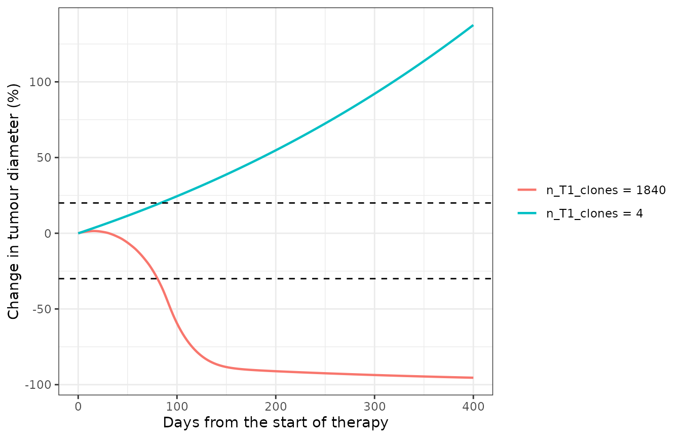
Nivolumab + entinostat in the reference patient at low and high tumour mutational burden. At high TMB the cancer cells are eliminated; the residual diameter is the minimum tumour-compartment volume plus the remaining T cells and dead-cell debris.
Nivolumab exposure
nivo <- arms |> filter(arm == "Nivolumab", day <= 140)
trough_ss <- nivo$Cc_nivolumab[nivo$day == 140] * mw[["nivolumab"]] / 1e6 # nmol/L -> ug/mL
trough_ss
#> [1] 64.68494
stopifnot(trough_ss > 20, trough_ss < 120)
The simulated nivolumab trough after 10 doses of 3 mg/kg every 2 weeks is about 65 ug/mL. The paper does not report nivolumab exposure, so this is a plausibility check only (tens of ug/mL for a therapeutic IgG4 regimen); the antibody PK parameters are those of Table S2, taken by the authors from Bajaj et al.
Mass conservation in the synapse
Receptor and ligand totals in each immunological synapse are conserved by the binding reactions (the antibodies are not consumed: SimBiology’s binding reactions list only the surface species). This is an exact identity of the ODE system, so it is checked tightly.
tri <- arms |> filter(arm == "Nivolumab + entinostat + ipilimumab")
pd1_tot <- with(tri, q_syn_T_C1_PD1 + q_syn_T_C1_PD1_PDL1 + q_syn_T_C1_PD1_PDL2 +
  q_syn_T_C1_PD1_nivo + 2 * q_syn_T_C1_PD1_nivo_PD1)
ctla4_tot <- with(tri, q_syn_T_APC_CTLA4 + q_syn_T_APC_CD80_CTLA4 + 2 * q_syn_T_APC_CTLA4_CD80_CTLA4 +
  2 * q_syn_T_APC_CD80_CTLA4_CD80_CTLA4 + q_syn_T_APC_CD80_CTLA4_CD80 + q_syn_T_APC_CD86_CTLA4 +
  q_syn_T_APC_CD86_CTLA4_CD86 + q_syn_T_APC_CTLA4_ipi + 2 * q_syn_T_APC_CTLA4_ipi_CTLA4)
pd1_0 <- 60000 / 151.31041193043737 * 37.8 # T_PD1_total / A_Tcell * synapse area
ctla4_0 <- 400 # T_CTLA4_syn / A_syn * synapse area
c(pd1 = max(abs(pd1_tot / pd1_0 - 1)), ctla4 = max(abs(ctla4_tot / ctla4_0 - 1)))
#>          pd1        ctla4
#> 2.900791e-12 2.537304e-11
stopifnot(max(abs(pd1_tot / pd1_0 - 1)) < 1e-4, max(abs(ctla4_tot / ctla4_0 - 1)) < 1e-4)
Assumptions and deviations
-
Values that differ between Table S2 and the SBML
deposit. Table S2 is used, with the SBML value noted in the
parameter’s comment:
k_Treg= 1/day (SBML: 2/day; Table S2 range 0.1-1, which excludes 2),IC50_ENT_ArgI= 5e-7 M (SBML: 3.74e-7 M; Table S7 also prints 5e-7 M),k_a2_ENT= 2.47/h (SBML: 2.5/h).k_cln_ENTuses the full-precision SBML value 1.22207654715555e-4 M/h, which Table S2 prints rounded as 1.22e-4. -
Durvalumab distribution and clearance. Table S2
prints
q_P_durv,q_T_durv,q_LN_durvandk_cl_durvin 1/second, which is dimensionally inconsistent with the rate laws (they multiply a concentration and must give an amount per time). The SBML deposit’s values (the nivolumab-like volumetric flows and a clearance of 0.4 L/day) are used. Durvalumab is not dosed in the paper, so this affects no published result. -
Entinostat buccal fraction.
F_ENT_buccal= 0.324 is not printed; it was back-solved by the maintainers from the published Cmax. The published AUC and the 10-h gastrointestinal peak of Figure 2B are not reproduced with the printed clearance (see the entinostat section); a 0.4-fold Michaelis-Menten capacity would reproduce them, but that is not the printed value and is not used. -
Cancer-cell elimination event (Table S6).
SimBiology resets the cancer cell count to zero when it falls below 0.9
cells. rxode2 has no state-reset events, so the model switches
proliferation off below 0.9 cells (
c1_alive); the remaining fraction of a cell then decays through the death terms instead of vanishing instantly. Tumour regrowth after elimination is prevented in both cases. -
Units. Arginase-I is carried in the export’s
placeholder unit mU, which SimBiology defines as 1 mol/L; the conversion
is kept exactly as exported, so
IC50_ArgI_CTL,EC50_ArgI_Tregandk_sec_ArgIkeep their printed relationship. - Dosing assumptions of this vignette. Body weight 70 kg for the mg/kg antibody doses (the paper sizes V_C and V_P “based on patient weight” but does not print the weight); molecular weights 146 kDa (nivolumab), 148 kDa (ipilimumab) and 376.41 g/mol (entinostat); antibodies given as IV boluses (the infusion duration is not stated).
- Reference patient. The pre-treatment diameter of 2.5 cm is a choice within the Table S2 range; the paper’s own response rates come from 1196 sampled parameter sets whose sampling distributions are not stated beyond their ranges, so they are not re-simulated here.
-
State names. The states keep the SimBiology
compartment.speciesnaming (q_V_T_C1,q_syn_T_C1_PD1, …) so each one can be traced to its Table S5 row; they are not mapped onto the library’s PK compartment names.