Isavuconazole (Desai 2016)
Source:vignettes/articles/Desai_2016_isavuconazole.Rmd
Desai_2016_isavuconazole.RmdModel and source
- Citation: Desai A, Schmitt-Hoffmann A-H, Mujais S, Townsend R. Population Pharmacokinetics of Isavuconazole in Subjects with Mild or Moderate Hepatic Impairment. Antimicrobial Agents and Chemotherapy. 2016;60(5):3025-3031. doi:10.1128/AAC.02942-15
- Description: Two-compartment population PK model for isavuconazole (administered as the prodrug isavuconazonium sulfate) in healthy adults and adults with mild (Child-Pugh A) or moderate (Child-Pugh B) hepatic impairment, following single 100 mg oral or 2-h intravenous doses (Desai 2016). Weibull absorption for the oral route; hepatic-impairment-group-specific typical CL and Q; linear BMI effect on peripheral volume.
- Article: https://doi.org/10.1128/AAC.02942-15 (open access, CC BY 4.0)
The Desai 2016 population PK model for isavuconazole was developed from two Phase 1 single-dose hepatic-impairment studies and is used here to simulate the clinical multiple-dose regimen and the trough concentrations reported in the source paper.
Population
The model was fit to 2,016 total isavuconazole plasma concentrations from 96 adults pooled across two Phase 1 studies (Desai 2016 Methods ‘Studies’ and Table 1). Each study enrolled 48 subjects: equal numbers of healthy controls, subjects with mild hepatic impairment (Child-Pugh Class A), and subjects with moderate hepatic impairment (Child-Pugh Class B). Study 1 sampled adults with alcoholic-cirrhosis-induced hepatic impairment; Study 2 sampled adults with chronic hepatitis B and/or C. Healthy controls were matched to impaired subjects on age (within +-7 years), sex, body weight (within +-8 kg), and BMI (within +-4 kg/m^2). Baseline demographics (Table 2): median age 50-54 years, median weight 76-78 kg, median BMI 26-28 kg/m^2, and 34% female across all strata. Mean Child-Pugh scores (Table 3) confirmed the mild stratum at 5.18 (alcoholic cirrhosis) / 5.75 (hepatitis B/C) and the moderate stratum at 7.43 / 8.31. Subjects received a single 100 mg isavuconazole equivalent (186 mg isavuconazonium sulfate) either orally (p.o.) or as a 2-hour intravenous infusion, with plasma sampling from predose to 480 hours postdose.
| field | value | |
|---|---|---|
| species | species | human |
| n_subjects | n_subjects | 96 |
| n_studies | n_studies | 2 |
| age_range | age_range | 37-64 years (median 50 healthy, 54 mild, 54 moderate per Table 2) |
| weight_range | weight_range | 53-107 kg (median 78 healthy, 76 mild, 76 moderate per Table 2) |
| bmi_range | bmi_range | 21-34 kg/m^2 (median 27 healthy, 28 mild, 26 moderate per Table 2) |
| sex_female_pct | sex_female_pct | 34 |
| disease_state | disease_state | Healthy controls and adults with mild (Child-Pugh A) or moderate (Child-Pugh B) hepatic impairment due to either alcoholic cirrhosis (Study 1, 48 subjects) or chronic hepatitis B/C (Study 2, 48 subjects). Equal n=32 in each of three hepatic-impairment strata. |
| hepatic_function | hepatic_function | Child-Pugh A (mild; mean composite score 5.18 alcoholic cirrhosis cohort / 5.75 hepatitis B/C cohort) and Child-Pugh B (moderate; mean 7.43 / 8.31). Healthy controls matched to impaired subjects on age (within +-7 years), sex, body weight (within +-8 kg), and BMI (within +-4 kg/m^2). See Table 3. |
| dose_range | dose_range | Single 100 mg isavuconazole equivalent (186 mg isavuconazonium sulfate prodrug) administered either orally (p.o.) or as a 2-h continuous intravenous infusion. |
| smoking_status | smoking_status | Healthy 59% smokers; mild 75%; moderate 75% (Table 2). |
| notes | notes | Data pooled across two Phase 1 single-dose hepatic-impairment studies for combined popPK analysis. Plasma sampling 0.5 to 480 h post-dose. 2,016 total isavuconazole plasma concentrations. Estimation in NONMEM 7.2 with FOCE method. Severe hepatic impairment (Child-Pugh C) was not studied. |
Source trace
The per-parameter origin is recorded as an in-file comment next to
each ini() entry in
inst/modeldb/specificDrugs/Desai_2016_isavuconazole.R. The
table below collects them in one place for review. All linear-scale
values in the paper’s Table 4 are reported in mL/h (CL, Q) and mL (V2,
V3); they are converted to L/h and L in the model file for consistency
with the nlmixr2lib units convention (time = h, concentration =
mg/L).
| Symbol in paper | Parameter in model | Value (paper / model) | Source location |
|---|---|---|---|
| theta_8 (CL healthy) | exp(lcl) |
2540 mL/h / 2.54 L/h | Table 4 |
| theta_1 (CL mild) | exp(lcl + e_hepimp_mild_cl) |
1550 mL/h / 1.55 L/h | Table 4 |
| theta_9 (CL moderate) | exp(lcl + e_hepimp_mod_cl) |
1326 mL/h / 1.326 L/h | Table 4 |
| theta_2 (V2) | exp(lvc) |
51,400 mL / 51.4 L | Table 4 |
| theta_10 (Q healthy) | exp(lq) |
33,678 mL/h / 33.678 L/h | Table 4 |
| theta_3 (Q mild) | exp(lq + e_hepimp_mild_q) |
38,800 mL/h / 38.8 L/h | Table 4 |
| theta_11 (Q moderate) | exp(lq + e_hepimp_mod_q) |
63,554 mL/h / 63.554 L/h | Table 4 |
| theta_4 (V3) | exp(lvp) |
410,000 mL / 410 L | Table 4 (printed as ‘41,0000’; bootstrap mean 410,661 mL confirms 410 L) |
| theta_5 (RA) | exp(lra) |
0.653 1/h | Table 4 |
| theta_6 (GAM1) | exp(lgam1) |
4.57 unitless | Table 4 |
| theta_7 (KAMAX) | exp(lkamax) |
0.86 1/h | Table 4 |
| theta_12 (BMI on V3) | e_bmi_vp |
0.058 per kg/m^2 | Table 4 and best-covariate model equation on p. 3028 |
| F1 |
exp(lfdepot) (fixed) |
1.00 fraction | Table 4 (‘F1 = 1.00 (fixed)’) |
| omega^2 (CL) | etalcl |
43.47% CV -> 0.17315 | Table 4 Variability section |
| omega^2 (V2) | etalvc |
21.23% CV -> 0.04408 | Table 4 Variability section |
| omega^2 (RA) | etalra |
32.55% CV -> 0.10070 | Table 4 Variability section |
| omega^2 (KAMAX) | etalkamax |
31.78% CV -> 0.09621 | Table 4 Variability section |
| omega^2 (GAM1) | etalgam1 |
38.07% CV -> 0.13534 | Table 4 Variability section |
| omega^2 (V3) | etalvp |
27.05% CV -> 0.07061 | Table 4 Variability section |
| omega^2 (Q) | etalq |
36.46% CV -> 0.12480 | Table 4 Variability section |
| sigma (residual) | propSd |
17.88% CV / 0.1788 | Table 4 ‘Residual error sigma^2 = 17.88’ |
| Best covariate model |
cl, q log-additive shifts, vp
linear-deviation BMI |
(see equation) | Best-covariate model equation on p. 3028 |
| Weibull ka(t) form | ka <- kamax * (1 - exp(-(ra * tad)^gam1)) |
Piotrovskij saturating-ka | Operator-approved interpretation (sidecar request-001 q3 = A); paper text names the three parameters but does not write the equation |
Virtual cohort
The original observational data are not publicly available. Two simulation exercises follow:
- Single-dose NCA validation. Three hepatic-impairment strata (healthy / mild / moderate) crossed with two routes (p.o. / 2-h i.v. infusion), each with 100 simulated subjects, replicating the paper’s data set design at the 100 mg single-dose level.
- Clinical multiple-dose simulation. The 200 mg every-8-hours x 2-day loading-and-maintenance regimen recommended in the prescribing information and used by the paper’s Monte Carlo simulation (Methods ‘Simulations’ and Figure 3), continued at 200 mg once daily through steady state. The simulated mean trough concentrations at steady state are compared against Table 5.
set.seed(20260609)

# Per-stratum number of subjects in each cohort. Setting to 100 gives a
# narrow-enough quantile band for the trough comparison without inflating
# vignette wall-time.
n_per <- 100

# BMI covariate is sampled from the pooled-cohort range (Table 2: median 27,
# range 21-34, taken approximately uniform across the three strata). For the
# typical-value reproduction of Figure 3 we hold BMI fixed at the reference
# 27 kg/m^2; for the NCA validation we let BMI vary as in the paper.
sample_bmi <- function(n) round(runif(n, 21, 34), 1)

make_cohort <- function(n, hep_mild, hep_mod, route, dose_mg, id_offset = 0L) {
  ids <- id_offset + seq_len(n)
  cov <- tibble(
    id = ids,
    BMI = sample_bmi(n),
    HEPIMP_MILD = hep_mild,
    HEPIMP_MOD  = hep_mod,
    stratum = if (hep_mod == 1) "moderate" else if (hep_mild == 1) "mild" else "healthy",
    route   = route
  )
  if (route == "po") {
    dose_row <- tibble(
      id = ids, time = 0, amt = dose_mg, rate = 0, cmt = "depot", evid = 1L, Cc = NA_real_
    )
  } else {
    # 2-h i.v. infusion: amt = dose_mg over 2 h -> rate = dose_mg / 2
    dose_row <- tibble(
      id = ids, time = 0, amt = dose_mg, rate = dose_mg / 2, cmt = "central", evid = 1L, Cc = NA_real_
    )
  }
  obs_times <- c(0.5, 1, 2, 3, 4, 6, 8, 10, 24, 48, 72, 96, 120, 144, 168, 216, 288, 360, 432, 480)
  obs <- tidyr::expand_grid(id = ids, time = obs_times) |>
    dplyr::mutate(amt = 0, rate = 0, cmt = "central", evid = 0L, Cc = NA_real_)
  dplyr::bind_rows(dose_row, obs) |>
    dplyr::left_join(cov, by = "id") |>
    dplyr::arrange(id, time, dplyr::desc(evid))
}

events_single <- dplyr::bind_rows(
  make_cohort(n_per, 0, 0, "po", 100, id_offset = 0L),
  make_cohort(n_per, 1, 0, "po", 100, id_offset = 1 * n_per),
  make_cohort(n_per, 0, 1, "po", 100, id_offset = 2 * n_per),
  make_cohort(n_per, 0, 0, "iv", 100, id_offset = 3 * n_per),
  make_cohort(n_per, 1, 0, "iv", 100, id_offset = 4 * n_per),
  make_cohort(n_per, 0, 1, "iv", 100, id_offset = 5 * n_per)
)
stopifnot(!anyDuplicated(unique(events_single[, c("id", "time", "evid")])))
events_single$treatment <- paste(events_single$route, events_single$stratum, sep = "_")
Simulation
mod <- readModelDb("Desai_2016_isavuconazole")
sim_single <- rxode2::rxSolve(
  mod, events = events_single,
  keep = c("stratum", "route", "treatment", "BMI", "HEPIMP_MILD", "HEPIMP_MOD")
)
#> ℹ parameter labels from comments will be replaced by 'label()'
sim_single <- as.data.frame(sim_single)
A typical-value (zeroRe) reproduction is used for the
Figure 3 replicate so the comparison against the paper’s mean profiles
is not blurred by IIV.
mod_typ <- mod |> rxode2::zeroRe()
#> ℹ parameter labels from comments will be replaced by 'label()'

# Reference cohort for Figure 3 / Table 5: healthy / mild / moderate adults at
# the reference BMI of 27 kg/m^2 on the clinical dosing regimen:
# 200 mg q8h x 2 days (6 loading doses) then 200 mg q24h.
# The simulation runs to day 28 because isavuconazole has a long terminal
# half-life (terminal t1/2 dominated by peripheral redistribution; Vp = 410 L,
# CL = 1.3-2.5 L/h gives lambda_z ~ 0.005-0.006 /h, t1/2 ~ 5 days). Day 14
# (the paper's nominal evaluation horizon) is only ~84% of steady state; day
# 28 reaches > 98% so the trough comparison against Table 5 is meaningful.
sim_horizon_h <- 28 * 24
load_times      <- seq(0, 48 - 8, by = 8)   # 0, 8, 16, 24, 32, 40
maintenance_t   <- seq(48, sim_horizon_h, by = 24)
dose_times      <- c(load_times, maintenance_t)
make_md_events <- function(stratum, hep_mild, hep_mod, id) {
  obs_times <- seq(0, sim_horizon_h, by = 0.5)
  doses <- tibble(id = id, time = dose_times, amt = 200, rate = 0,
                  cmt = "depot", evid = 1L, Cc = NA_real_)
  obs <- tibble(id = id, time = obs_times, amt = 0, rate = 0,
                cmt = "central", evid = 0L, Cc = NA_real_)
  dplyr::bind_rows(doses, obs) |>
    dplyr::mutate(BMI = 27, HEPIMP_MILD = hep_mild, HEPIMP_MOD = hep_mod,
                  stratum = stratum) |>
    dplyr::arrange(time, dplyr::desc(evid))
}
events_typ <- dplyr::bind_rows(
  make_md_events("healthy",  0, 0, id = 1L),
  make_md_events("mild",     1, 0, id = 2L),
  make_md_events("moderate", 0, 1, id = 3L)
)
sim_typ <- rxode2::rxSolve(mod_typ, events = events_typ, keep = "stratum")
#> ℹ omega/sigma items treated as zero: 'etalcl', 'etalvc', 'etalra', 'etalkamax', 'etalgam1', 'etalvp', 'etalq'
#> Warning: multi-subject simulation without without 'omega'
sim_typ <- as.data.frame(sim_typ)
Replicate published figures
# Replicates Figure 3 of Desai 2016: mean simulated isavuconazole
# concentrations under the clinical 200 mg q8h x 2 days then 200 mg q24h
# regimen, by hepatic-impairment stratum. Figure 3 shows ng/mL on a linear
# scale; the conversion factor is 1 mg/L = 1000 ng/mL.
sim_typ |>
  dplyr::filter(time > 0) |>
  dplyr::mutate(Cc_ng_per_mL = Cc * 1000,
                stratum = factor(stratum, levels = c("healthy", "mild", "moderate"))) |>
  ggplot(aes(time / 24, Cc_ng_per_mL, color = stratum)) +
  geom_line(linewidth = 0.7) +
  scale_color_manual(values = c(healthy = "#1f77b4", mild = "#2ca02c", moderate = "#d62728")) +
  labs(x = "Time after first dose (days)", y = "Isavuconazole (ng/mL)",
       color = "Hepatic impairment",
       title = "Figure 3 -- typical-value simulation under the clinical 200 mg q8h x 2 d then 200 mg q24h regimen",
       caption = "Replicates Figure 3 of Desai 2016 (mean simulated concentrations vs time across the three strata).")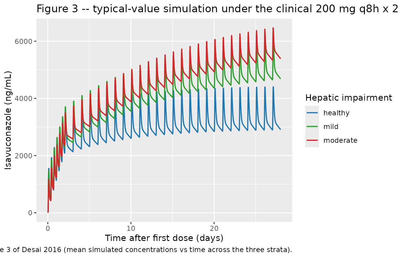
# Stochastic VPC of the same regimen using the full IIV; compare to the 95% CI
# band that the paper overlays on Figure 3 plus the Table 5 Monte Carlo mean
# trough.
n_vpc <- 200
vpc_cohorts <- dplyr::bind_rows(
  make_cohort(n_vpc, 0, 0, "po", 200, id_offset = 0L) |>
    dplyr::mutate(stratum = "healthy"),
  make_cohort(n_vpc, 1, 0, "po", 200, id_offset = 1 * n_vpc) |>
    dplyr::mutate(stratum = "mild"),
  make_cohort(n_vpc, 0, 1, "po", 200, id_offset = 2 * n_vpc) |>
    dplyr::mutate(stratum = "moderate")
)
# Replace the single 100 mg single-dose row with the q8h / q24h regimen run to
# the same 28-day horizon as the typical-value simulation so trough sampling
# at day 28 is past steady state.
vpc_doses <- vpc_cohorts |>
  dplyr::filter(evid == 1L) |>
  dplyr::select(id, BMI, HEPIMP_MILD, HEPIMP_MOD, stratum, route) |>
  dplyr::distinct() |>
  tidyr::expand_grid(dose_time = dose_times) |>
  dplyr::transmute(id, time = dose_time, amt = 200, rate = 0,
                   cmt = "depot", evid = 1L, Cc = NA_real_,
                   BMI, HEPIMP_MILD, HEPIMP_MOD, stratum, route)
vpc_obs <- vpc_cohorts |>
  dplyr::filter(evid == 0L) |>
  dplyr::select(id, BMI, HEPIMP_MILD, HEPIMP_MOD, stratum, route) |>
  dplyr::distinct() |>
  tidyr::expand_grid(time = seq(0, sim_horizon_h, by = 4)) |>
  dplyr::transmute(id, time, amt = 0, rate = 0, cmt = "central", evid = 0L, Cc = NA_real_,
                   BMI, HEPIMP_MILD, HEPIMP_MOD, stratum, route)
events_vpc <- dplyr::bind_rows(vpc_doses, vpc_obs) |>
  dplyr::arrange(id, time, dplyr::desc(evid))
stopifnot(!anyDuplicated(unique(events_vpc[, c("id", "time", "evid")])))

sim_vpc <- rxode2::rxSolve(mod, events = events_vpc, keep = c("stratum"))
#> ℹ parameter labels from comments will be replaced by 'label()'
sim_vpc <- as.data.frame(sim_vpc)

sim_vpc |>
  dplyr::filter(time > 0, !is.na(Cc)) |>
  dplyr::mutate(Cc_ng_per_mL = Cc * 1000) |>
  dplyr::group_by(stratum, time) |>
  dplyr::summarise(
    Q05 = quantile(Cc_ng_per_mL, 0.05, na.rm = TRUE),
    Q50 = quantile(Cc_ng_per_mL, 0.50, na.rm = TRUE),
    Q95 = quantile(Cc_ng_per_mL, 0.95, na.rm = TRUE),
    .groups = "drop"
  ) |>
  dplyr::mutate(stratum = factor(stratum, levels = c("healthy", "mild", "moderate"))) |>
  ggplot(aes(time / 24, Q50, color = stratum, fill = stratum)) +
  geom_ribbon(aes(ymin = Q05, ymax = Q95), color = NA, alpha = 0.20) +
  geom_line(linewidth = 0.6) +
  facet_wrap(~stratum) +
  scale_color_manual(values = c(healthy = "#1f77b4", mild = "#2ca02c", moderate = "#d62728")) +
  scale_fill_manual(values = c(healthy = "#1f77b4", mild = "#2ca02c", moderate = "#d62728")) +
  labs(x = "Time after first dose (days)", y = "Isavuconazole (ng/mL)",
       title = "Stochastic VPC of the clinical regimen by hepatic-impairment stratum",
       caption = "Median (line) and 5th-95th percentile band (shaded) from 200 virtual subjects per stratum.")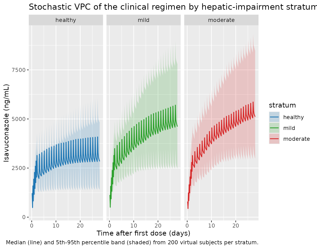
PKNCA validation
PKNCA computes NCA parameters for the single-dose 100 mg p.o. and
i.v. treatments that match the paper’s source data. Cmax, Tmax, AUC, and
half-life are summarised per treatment (route x stratum) so
each can be inspected against the paper’s reported population mean
clearance values (Abstract; mean CL: 2.5 L/h healthy, 1.55 L/h mild,
1.32 L/h moderate).
sim_nca <- sim_single |>
  dplyr::filter(!is.na(Cc), time > 0) |>
  dplyr::select(id, time, Cc, treatment, route, stratum)

dose_df <- events_single |>
  dplyr::filter(evid == 1L) |>
  dplyr::select(id, time, amt, treatment, route, stratum)

conc_obj <- PKNCA::PKNCAconc(sim_nca, Cc ~ time | treatment + id,
                             concu = "mg/L", timeu = "hr")
dose_obj <- PKNCA::PKNCAdose(dose_df, amt ~ time | treatment + id,
                             doseu = "mg")
#> Found column named route, using it for the attribute of the same name.

intervals <- data.frame(
  start       = 0,
  end         = Inf,
  cmax        = TRUE,
  tmax        = TRUE,
  aucinf.obs  = TRUE,
  half.life   = TRUE,
  cl.obs      = TRUE
)

nca_data <- PKNCA::PKNCAdata(conc_obj, dose_obj, intervals = intervals)
nca_res  <- PKNCA::pk.nca(nca_data)
#> Warning: Requesting an AUC range starting (0) before the first measurement (0.5) is not allowed
#> Requesting an AUC range starting (0) before the first measurement (0.5) is not allowed
#> Requesting an AUC range starting (0) before the first measurement (0.5) is not allowed
#> Requesting an AUC range starting (0) before the first measurement (0.5) is not allowed
#> Requesting an AUC range starting (0) before the first measurement (0.5) is not allowed
#> Requesting an AUC range starting (0) before the first measurement (0.5) is not allowed
#> Requesting an AUC range starting (0) before the first measurement (0.5) is not allowed
#> Requesting an AUC range starting (0) before the first measurement (0.5) is not allowed
#> Requesting an AUC range starting (0) before the first measurement (0.5) is not allowed
#> Requesting an AUC range starting (0) before the first measurement (0.5) is not allowed
#> Requesting an AUC range starting (0) before the first measurement (0.5) is not allowed
#> Requesting an AUC range starting (0) before the first measurement (0.5) is not allowed
#> Requesting an AUC range starting (0) before the first measurement (0.5) is not allowed
#> Requesting an AUC range starting (0) before the first measurement (0.5) is not allowed
#> Requesting an AUC range starting (0) before the first measurement (0.5) is not allowed
#> Requesting an AUC range starting (0) before the first measurement (0.5) is not allowed
#> Requesting an AUC range starting (0) before the first measurement (0.5) is not allowed
#> Requesting an AUC range starting (0) before the first measurement (0.5) is not allowed
#> Requesting an AUC range starting (0) before the first measurement (0.5) is not allowed
#> Requesting an AUC range starting (0) before the first measurement (0.5) is not allowed
#> Requesting an AUC range starting (0) before the first measurement (0.5) is not allowed
#> Requesting an AUC range starting (0) before the first measurement (0.5) is not allowed
#> Requesting an AUC range starting (0) before the first measurement (0.5) is not allowed
#> Requesting an AUC range starting (0) before the first measurement (0.5) is not allowed
#> Requesting an AUC range starting (0) before the first measurement (0.5) is not allowed
#> Requesting an AUC range starting (0) before the first measurement (0.5) is not allowed
#> Requesting an AUC range starting (0) before the first measurement (0.5) is not allowed
#> Requesting an AUC range starting (0) before the first measurement (0.5) is not allowed
#> Requesting an AUC range starting (0) before the first measurement (0.5) is not allowed
#> Requesting an AUC range starting (0) before the first measurement (0.5) is not allowed
#> Requesting an AUC range starting (0) before the first measurement (0.5) is not allowed
#> Requesting an AUC range starting (0) before the first measurement (0.5) is not allowed
#> Requesting an AUC range starting (0) before the first measurement (0.5) is not allowed
#> Requesting an AUC range starting (0) before the first measurement (0.5) is not allowed
#> Requesting an AUC range starting (0) before the first measurement (0.5) is not allowed
#> Requesting an AUC range starting (0) before the first measurement (0.5) is not allowed
#> Requesting an AUC range starting (0) before the first measurement (0.5) is not allowed
#> Requesting an AUC range starting (0) before the first measurement (0.5) is not allowed
#> Requesting an AUC range starting (0) before the first measurement (0.5) is not allowed
#> Requesting an AUC range starting (0) before the first measurement (0.5) is not allowed
#> Requesting an AUC range starting (0) before the first measurement (0.5) is not allowed
#> Requesting an AUC range starting (0) before the first measurement (0.5) is not allowed
#> Requesting an AUC range starting (0) before the first measurement (0.5) is not allowed
#> Requesting an AUC range starting (0) before the first measurement (0.5) is not allowed
#> Requesting an AUC range starting (0) before the first measurement (0.5) is not allowed
#> Requesting an AUC range starting (0) before the first measurement (0.5) is not allowed
#> Requesting an AUC range starting (0) before the first measurement (0.5) is not allowed
#> Requesting an AUC range starting (0) before the first measurement (0.5) is not allowed
#> Requesting an AUC range starting (0) before the first measurement (0.5) is not allowed
#> Requesting an AUC range starting (0) before the first measurement (0.5) is not allowed
#> Requesting an AUC range starting (0) before the first measurement (0.5) is not allowed
#> Requesting an AUC range starting (0) before the first measurement (0.5) is not allowed
#> Requesting an AUC range starting (0) before the first measurement (0.5) is not allowed
#> Requesting an AUC range starting (0) before the first measurement (0.5) is not allowed
#> Requesting an AUC range starting (0) before the first measurement (0.5) is not allowed
#> Requesting an AUC range starting (0) before the first measurement (0.5) is not allowed
#> Requesting an AUC range starting (0) before the first measurement (0.5) is not allowed
#> Requesting an AUC range starting (0) before the first measurement (0.5) is not allowed
#> Requesting an AUC range starting (0) before the first measurement (0.5) is not allowed
#> Requesting an AUC range starting (0) before the first measurement (0.5) is not allowed
#> Requesting an AUC range starting (0) before the first measurement (0.5) is not allowed
#> Requesting an AUC range starting (0) before the first measurement (0.5) is not allowed
#> Requesting an AUC range starting (0) before the first measurement (0.5) is not allowed
#> Requesting an AUC range starting (0) before the first measurement (0.5) is not allowed
#> Requesting an AUC range starting (0) before the first measurement (0.5) is not allowed
#> Requesting an AUC range starting (0) before the first measurement (0.5) is not allowed
#> Requesting an AUC range starting (0) before the first measurement (0.5) is not allowed
#> Requesting an AUC range starting (0) before the first measurement (0.5) is not allowed
#> Requesting an AUC range starting (0) before the first measurement (0.5) is not allowed
#> Requesting an AUC range starting (0) before the first measurement (0.5) is not allowed
#> Requesting an AUC range starting (0) before the first measurement (0.5) is not allowed
#> Requesting an AUC range starting (0) before the first measurement (0.5) is not allowed
#> Requesting an AUC range starting (0) before the first measurement (0.5) is not allowed
#> Requesting an AUC range starting (0) before the first measurement (0.5) is not allowed
#> Requesting an AUC range starting (0) before the first measurement (0.5) is not allowed
#> Requesting an AUC range starting (0) before the first measurement (0.5) is not allowed
#> Requesting an AUC range starting (0) before the first measurement (0.5) is not allowed
#> Requesting an AUC range starting (0) before the first measurement (0.5) is not allowed
#> Requesting an AUC range starting (0) before the first measurement (0.5) is not allowed
#> Requesting an AUC range starting (0) before the first measurement (0.5) is not allowed
#> Requesting an AUC range starting (0) before the first measurement (0.5) is not allowed
#> Requesting an AUC range starting (0) before the first measurement (0.5) is not allowed
#> Requesting an AUC range starting (0) before the first measurement (0.5) is not allowed
#> Requesting an AUC range starting (0) before the first measurement (0.5) is not allowed
#> Requesting an AUC range starting (0) before the first measurement (0.5) is not allowed
#> Requesting an AUC range starting (0) before the first measurement (0.5) is not allowed
#> Requesting an AUC range starting (0) before the first measurement (0.5) is not allowed
#> Requesting an AUC range starting (0) before the first measurement (0.5) is not allowed
#> Requesting an AUC range starting (0) before the first measurement (0.5) is not allowed
#> Requesting an AUC range starting (0) before the first measurement (0.5) is not allowed
#> Requesting an AUC range starting (0) before the first measurement (0.5) is not allowed
#> Requesting an AUC range starting (0) before the first measurement (0.5) is not allowed
#> Requesting an AUC range starting (0) before the first measurement (0.5) is not allowed
#> Requesting an AUC range starting (0) before the first measurement (0.5) is not allowed
#> Requesting an AUC range starting (0) before the first measurement (0.5) is not allowed
#> Requesting an AUC range starting (0) before the first measurement (0.5) is not allowed
#> Requesting an AUC range starting (0) before the first measurement (0.5) is not allowed
#> Requesting an AUC range starting (0) before the first measurement (0.5) is not allowed
#> Requesting an AUC range starting (0) before the first measurement (0.5) is not allowed
#> Requesting an AUC range starting (0) before the first measurement (0.5) is not allowed
#> Requesting an AUC range starting (0) before the first measurement (0.5) is not allowed
#> Requesting an AUC range starting (0) before the first measurement (0.5) is not allowed
#> Requesting an AUC range starting (0) before the first measurement (0.5) is not allowed
#> Requesting an AUC range starting (0) before the first measurement (0.5) is not allowed
#> Requesting an AUC range starting (0) before the first measurement (0.5) is not allowed
#> Requesting an AUC range starting (0) before the first measurement (0.5) is not allowed
#> Requesting an AUC range starting (0) before the first measurement (0.5) is not allowed
#> Requesting an AUC range starting (0) before the first measurement (0.5) is not allowed
#> Requesting an AUC range starting (0) before the first measurement (0.5) is not allowed
#> Requesting an AUC range starting (0) before the first measurement (0.5) is not allowed
#> Requesting an AUC range starting (0) before the first measurement (0.5) is not allowed
#> Requesting an AUC range starting (0) before the first measurement (0.5) is not allowed
#> Requesting an AUC range starting (0) before the first measurement (0.5) is not allowed
#> Requesting an AUC range starting (0) before the first measurement (0.5) is not allowed
#> Requesting an AUC range starting (0) before the first measurement (0.5) is not allowed
#> Requesting an AUC range starting (0) before the first measurement (0.5) is not allowed
#> Requesting an AUC range starting (0) before the first measurement (0.5) is not allowed
#> Requesting an AUC range starting (0) before the first measurement (0.5) is not allowed
#> Requesting an AUC range starting (0) before the first measurement (0.5) is not allowed
#> Requesting an AUC range starting (0) before the first measurement (0.5) is not allowed
#> Requesting an AUC range starting (0) before the first measurement (0.5) is not allowed
#> Requesting an AUC range starting (0) before the first measurement (0.5) is not allowed
#> Requesting an AUC range starting (0) before the first measurement (0.5) is not allowed
#> Requesting an AUC range starting (0) before the first measurement (0.5) is not allowed
#> Requesting an AUC range starting (0) before the first measurement (0.5) is not allowed
#> Requesting an AUC range starting (0) before the first measurement (0.5) is not allowed
#> Requesting an AUC range starting (0) before the first measurement (0.5) is not allowed
#> Requesting an AUC range starting (0) before the first measurement (0.5) is not allowed
#> Requesting an AUC range starting (0) before the first measurement (0.5) is not allowed
#> Requesting an AUC range starting (0) before the first measurement (0.5) is not allowed
#> Requesting an AUC range starting (0) before the first measurement (0.5) is not allowed
#> Requesting an AUC range starting (0) before the first measurement (0.5) is not allowed
#> Requesting an AUC range starting (0) before the first measurement (0.5) is not allowed
#> Requesting an AUC range starting (0) before the first measurement (0.5) is not allowed
#> Requesting an AUC range starting (0) before the first measurement (0.5) is not allowed
#> Requesting an AUC range starting (0) before the first measurement (0.5) is not allowed
#> Requesting an AUC range starting (0) before the first measurement (0.5) is not allowed
#> Requesting an AUC range starting (0) before the first measurement (0.5) is not allowed
#> Requesting an AUC range starting (0) before the first measurement (0.5) is not allowed
#> Requesting an AUC range starting (0) before the first measurement (0.5) is not allowed
#> Requesting an AUC range starting (0) before the first measurement (0.5) is not allowed
#> Requesting an AUC range starting (0) before the first measurement (0.5) is not allowed
#> Requesting an AUC range starting (0) before the first measurement (0.5) is not allowed
#> Requesting an AUC range starting (0) before the first measurement (0.5) is not allowed
#> Requesting an AUC range starting (0) before the first measurement (0.5) is not allowed
#> Requesting an AUC range starting (0) before the first measurement (0.5) is not allowed
#> Requesting an AUC range starting (0) before the first measurement (0.5) is not allowed
#> Requesting an AUC range starting (0) before the first measurement (0.5) is not allowed
#> Requesting an AUC range starting (0) before the first measurement (0.5) is not allowed
#> Requesting an AUC range starting (0) before the first measurement (0.5) is not allowed
#> Requesting an AUC range starting (0) before the first measurement (0.5) is not allowed
#> Requesting an AUC range starting (0) before the first measurement (0.5) is not allowed
#> Requesting an AUC range starting (0) before the first measurement (0.5) is not allowed
#> Requesting an AUC range starting (0) before the first measurement (0.5) is not allowed
#> Requesting an AUC range starting (0) before the first measurement (0.5) is not allowed
#> Requesting an AUC range starting (0) before the first measurement (0.5) is not allowed
#> Requesting an AUC range starting (0) before the first measurement (0.5) is not allowed
#> Requesting an AUC range starting (0) before the first measurement (0.5) is not allowed
#> Requesting an AUC range starting (0) before the first measurement (0.5) is not allowed
#> Requesting an AUC range starting (0) before the first measurement (0.5) is not allowed
#> Requesting an AUC range starting (0) before the first measurement (0.5) is not allowed
#> Requesting an AUC range starting (0) before the first measurement (0.5) is not allowed
#> Requesting an AUC range starting (0) before the first measurement (0.5) is not allowed
#> Requesting an AUC range starting (0) before the first measurement (0.5) is not allowed
#> Requesting an AUC range starting (0) before the first measurement (0.5) is not allowed
#> Requesting an AUC range starting (0) before the first measurement (0.5) is not allowed
#> Requesting an AUC range starting (0) before the first measurement (0.5) is not allowed
#> Requesting an AUC range starting (0) before the first measurement (0.5) is not allowed
#> Requesting an AUC range starting (0) before the first measurement (0.5) is not allowed
#> Requesting an AUC range starting (0) before the first measurement (0.5) is not allowed
#> Requesting an AUC range starting (0) before the first measurement (0.5) is not allowed
#> Requesting an AUC range starting (0) before the first measurement (0.5) is not allowed
#> Requesting an AUC range starting (0) before the first measurement (0.5) is not allowed
#> Requesting an AUC range starting (0) before the first measurement (0.5) is not allowed
#> Requesting an AUC range starting (0) before the first measurement (0.5) is not allowed
#> Requesting an AUC range starting (0) before the first measurement (0.5) is not allowed
#> Requesting an AUC range starting (0) before the first measurement (0.5) is not allowed
#> Requesting an AUC range starting (0) before the first measurement (0.5) is not allowed
#> Requesting an AUC range starting (0) before the first measurement (0.5) is not allowed
#> Requesting an AUC range starting (0) before the first measurement (0.5) is not allowed
#> Requesting an AUC range starting (0) before the first measurement (0.5) is not allowed
#> Requesting an AUC range starting (0) before the first measurement (0.5) is not allowed
#> Requesting an AUC range starting (0) before the first measurement (0.5) is not allowed
#> Requesting an AUC range starting (0) before the first measurement (0.5) is not allowed
#> Requesting an AUC range starting (0) before the first measurement (0.5) is not allowed
#> Requesting an AUC range starting (0) before the first measurement (0.5) is not allowed
#> Requesting an AUC range starting (0) before the first measurement (0.5) is not allowed
#> Requesting an AUC range starting (0) before the first measurement (0.5) is not allowed
#> Requesting an AUC range starting (0) before the first measurement (0.5) is not allowed
#> Requesting an AUC range starting (0) before the first measurement (0.5) is not allowed
#> Requesting an AUC range starting (0) before the first measurement (0.5) is not allowed
#> Requesting an AUC range starting (0) before the first measurement (0.5) is not allowed
#> Requesting an AUC range starting (0) before the first measurement (0.5) is not allowed
#> Requesting an AUC range starting (0) before the first measurement (0.5) is not allowed
#> Requesting an AUC range starting (0) before the first measurement (0.5) is not allowed
#> Requesting an AUC range starting (0) before the first measurement (0.5) is not allowed
#> Requesting an AUC range starting (0) before the first measurement (0.5) is not allowed
#> Requesting an AUC range starting (0) before the first measurement (0.5) is not allowed
#> Requesting an AUC range starting (0) before the first measurement (0.5) is not allowed
#> Requesting an AUC range starting (0) before the first measurement (0.5) is not allowed
#> Requesting an AUC range starting (0) before the first measurement (0.5) is not allowed
#> Requesting an AUC range starting (0) before the first measurement (0.5) is not allowed
#> Requesting an AUC range starting (0) before the first measurement (0.5) is not allowed
#> Requesting an AUC range starting (0) before the first measurement (0.5) is not allowed
#> Requesting an AUC range starting (0) before the first measurement (0.5) is not allowed
#> Requesting an AUC range starting (0) before the first measurement (0.5) is not allowed
#> Requesting an AUC range starting (0) before the first measurement (0.5) is not allowed
#> Requesting an AUC range starting (0) before the first measurement (0.5) is not allowed
#> Requesting an AUC range starting (0) before the first measurement (0.5) is not allowed
#> Requesting an AUC range starting (0) before the first measurement (0.5) is not allowed
#> Requesting an AUC range starting (0) before the first measurement (0.5) is not allowed
#> Requesting an AUC range starting (0) before the first measurement (0.5) is not allowed
#> Requesting an AUC range starting (0) before the first measurement (0.5) is not allowed
#> Requesting an AUC range starting (0) before the first measurement (0.5) is not allowed
#> Requesting an AUC range starting (0) before the first measurement (0.5) is not allowed
#> Requesting an AUC range starting (0) before the first measurement (0.5) is not allowed
#> Requesting an AUC range starting (0) before the first measurement (0.5) is not allowed
#> Requesting an AUC range starting (0) before the first measurement (0.5) is not allowed
#> Requesting an AUC range starting (0) before the first measurement (0.5) is not allowed
#> Requesting an AUC range starting (0) before the first measurement (0.5) is not allowed
#> Requesting an AUC range starting (0) before the first measurement (0.5) is not allowed
#> Requesting an AUC range starting (0) before the first measurement (0.5) is not allowed
#> Requesting an AUC range starting (0) before the first measurement (0.5) is not allowed
#> Requesting an AUC range starting (0) before the first measurement (0.5) is not allowed
#> Requesting an AUC range starting (0) before the first measurement (0.5) is not allowed
#> Requesting an AUC range starting (0) before the first measurement (0.5) is not allowed
#> Requesting an AUC range starting (0) before the first measurement (0.5) is not allowed
#> Requesting an AUC range starting (0) before the first measurement (0.5) is not allowed
#> Requesting an AUC range starting (0) before the first measurement (0.5) is not allowed
#> Requesting an AUC range starting (0) before the first measurement (0.5) is not allowed
#> Requesting an AUC range starting (0) before the first measurement (0.5) is not allowed
#> Requesting an AUC range starting (0) before the first measurement (0.5) is not allowed
#> Requesting an AUC range starting (0) before the first measurement (0.5) is not allowed
#> Requesting an AUC range starting (0) before the first measurement (0.5) is not allowed
#> Requesting an AUC range starting (0) before the first measurement (0.5) is not allowed
#> Requesting an AUC range starting (0) before the first measurement (0.5) is not allowed
#> Requesting an AUC range starting (0) before the first measurement (0.5) is not allowed
#> Requesting an AUC range starting (0) before the first measurement (0.5) is not allowed
#> Requesting an AUC range starting (0) before the first measurement (0.5) is not allowed
#> Requesting an AUC range starting (0) before the first measurement (0.5) is not allowed
#> Requesting an AUC range starting (0) before the first measurement (0.5) is not allowed
#> Requesting an AUC range starting (0) before the first measurement (0.5) is not allowed
#> Requesting an AUC range starting (0) before the first measurement (0.5) is not allowed
#> Requesting an AUC range starting (0) before the first measurement (0.5) is not allowed
#> Requesting an AUC range starting (0) before the first measurement (0.5) is not allowed
#> Requesting an AUC range starting (0) before the first measurement (0.5) is not allowed
#> Requesting an AUC range starting (0) before the first measurement (0.5) is not allowed
#> Requesting an AUC range starting (0) before the first measurement (0.5) is not allowed
#> Requesting an AUC range starting (0) before the first measurement (0.5) is not allowed
#> Requesting an AUC range starting (0) before the first measurement (0.5) is not allowed
#> Requesting an AUC range starting (0) before the first measurement (0.5) is not allowed
#> Requesting an AUC range starting (0) before the first measurement (0.5) is not allowed
#> Requesting an AUC range starting (0) before the first measurement (0.5) is not allowed
#> Requesting an AUC range starting (0) before the first measurement (0.5) is not allowed
#> Requesting an AUC range starting (0) before the first measurement (0.5) is not allowed
#> Requesting an AUC range starting (0) before the first measurement (0.5) is not allowed
#> Requesting an AUC range starting (0) before the first measurement (0.5) is not allowed
#> Requesting an AUC range starting (0) before the first measurement (0.5) is not allowed
#> Requesting an AUC range starting (0) before the first measurement (0.5) is not allowed
#> Requesting an AUC range starting (0) before the first measurement (0.5) is not allowed
#> Requesting an AUC range starting (0) before the first measurement (0.5) is not allowed
#> Requesting an AUC range starting (0) before the first measurement (0.5) is not allowed
#> Requesting an AUC range starting (0) before the first measurement (0.5) is not allowed
#> Requesting an AUC range starting (0) before the first measurement (0.5) is not allowed
#> Requesting an AUC range starting (0) before the first measurement (0.5) is not allowed
#> Requesting an AUC range starting (0) before the first measurement (0.5) is not allowed
#> Requesting an AUC range starting (0) before the first measurement (0.5) is not allowed
#> Requesting an AUC range starting (0) before the first measurement (0.5) is not allowed
#> Requesting an AUC range starting (0) before the first measurement (0.5) is not allowed
#> Requesting an AUC range starting (0) before the first measurement (0.5) is not allowed
#> Requesting an AUC range starting (0) before the first measurement (0.5) is not allowed
#> Requesting an AUC range starting (0) before the first measurement (0.5) is not allowed
#> Requesting an AUC range starting (0) before the first measurement (0.5) is not allowed
#> Requesting an AUC range starting (0) before the first measurement (0.5) is not allowed
#> Requesting an AUC range starting (0) before the first measurement (0.5) is not allowed
#> Requesting an AUC range starting (0) before the first measurement (0.5) is not allowed
#> Requesting an AUC range starting (0) before the first measurement (0.5) is not allowed
#> Requesting an AUC range starting (0) before the first measurement (0.5) is not allowed
#> Requesting an AUC range starting (0) before the first measurement (0.5) is not allowed
#> Requesting an AUC range starting (0) before the first measurement (0.5) is not allowed
#> Requesting an AUC range starting (0) before the first measurement (0.5) is not allowed
#> Requesting an AUC range starting (0) before the first measurement (0.5) is not allowed
#> Requesting an AUC range starting (0) before the first measurement (0.5) is not allowed
#> Requesting an AUC range starting (0) before the first measurement (0.5) is not allowed
#> Requesting an AUC range starting (0) before the first measurement (0.5) is not allowed
#> Requesting an AUC range starting (0) before the first measurement (0.5) is not allowed
#> Requesting an AUC range starting (0) before the first measurement (0.5) is not allowed
#> Requesting an AUC range starting (0) before the first measurement (0.5) is not allowed
#> Requesting an AUC range starting (0) before the first measurement (0.5) is not allowed
#> Requesting an AUC range starting (0) before the first measurement (0.5) is not allowed
#> Requesting an AUC range starting (0) before the first measurement (0.5) is not allowed
#> Requesting an AUC range starting (0) before the first measurement (0.5) is not allowed
#> Requesting an AUC range starting (0) before the first measurement (0.5) is not allowed
#> Requesting an AUC range starting (0) before the first measurement (0.5) is not allowed
#> Requesting an AUC range starting (0) before the first measurement (0.5) is not allowed
#> Requesting an AUC range starting (0) before the first measurement (0.5) is not allowed
#> Requesting an AUC range starting (0) before the first measurement (0.5) is not allowed
#> Requesting an AUC range starting (0) before the first measurement (0.5) is not allowed
#> Requesting an AUC range starting (0) before the first measurement (0.5) is not allowed
#> Requesting an AUC range starting (0) before the first measurement (0.5) is not allowed
#> Requesting an AUC range starting (0) before the first measurement (0.5) is not allowed
#> Requesting an AUC range starting (0) before the first measurement (0.5) is not allowed
#> Requesting an AUC range starting (0) before the first measurement (0.5) is not allowed
#> Requesting an AUC range starting (0) before the first measurement (0.5) is not allowed
#> Requesting an AUC range starting (0) before the first measurement (0.5) is not allowed
#> Requesting an AUC range starting (0) before the first measurement (0.5) is not allowed
#> Requesting an AUC range starting (0) before the first measurement (0.5) is not allowed
#> Requesting an AUC range starting (0) before the first measurement (0.5) is not allowed
#> Requesting an AUC range starting (0) before the first measurement (0.5) is not allowed
#> Requesting an AUC range starting (0) before the first measurement (0.5) is not allowed
#> Requesting an AUC range starting (0) before the first measurement (0.5) is not allowed
#> Requesting an AUC range starting (0) before the first measurement (0.5) is not allowed
#> Requesting an AUC range starting (0) before the first measurement (0.5) is not allowed
#> Requesting an AUC range starting (0) before the first measurement (0.5) is not allowed
#> Requesting an AUC range starting (0) before the first measurement (0.5) is not allowed
#> Requesting an AUC range starting (0) before the first measurement (0.5) is not allowed
#> Requesting an AUC range starting (0) before the first measurement (0.5) is not allowed
#> Requesting an AUC range starting (0) before the first measurement (0.5) is not allowed
#> Requesting an AUC range starting (0) before the first measurement (0.5) is not allowed
#> Requesting an AUC range starting (0) before the first measurement (0.5) is not allowed
#> Requesting an AUC range starting (0) before the first measurement (0.5) is not allowed
#> Requesting an AUC range starting (0) before the first measurement (0.5) is not allowed
#> Requesting an AUC range starting (0) before the first measurement (0.5) is not allowed
#> Requesting an AUC range starting (0) before the first measurement (0.5) is not allowed
#> Requesting an AUC range starting (0) before the first measurement (0.5) is not allowed
#> Requesting an AUC range starting (0) before the first measurement (0.5) is not allowed
#> Requesting an AUC range starting (0) before the first measurement (0.5) is not allowed
#> Requesting an AUC range starting (0) before the first measurement (0.5) is not allowed
#> Requesting an AUC range starting (0) before the first measurement (0.5) is not allowed
#> Requesting an AUC range starting (0) before the first measurement (0.5) is not allowed
#> Requesting an AUC range starting (0) before the first measurement (0.5) is not allowed
#> Requesting an AUC range starting (0) before the first measurement (0.5) is not allowed
#> Requesting an AUC range starting (0) before the first measurement (0.5) is not allowed
#> Requesting an AUC range starting (0) before the first measurement (0.5) is not allowed
#> Requesting an AUC range starting (0) before the first measurement (0.5) is not allowed
#> Requesting an AUC range starting (0) before the first measurement (0.5) is not allowed
#> Requesting an AUC range starting (0) before the first measurement (0.5) is not allowed
#> Requesting an AUC range starting (0) before the first measurement (0.5) is not allowed
#> Requesting an AUC range starting (0) before the first measurement (0.5) is not allowed
#> Requesting an AUC range starting (0) before the first measurement (0.5) is not allowed
#> Requesting an AUC range starting (0) before the first measurement (0.5) is not allowed
#> Requesting an AUC range starting (0) before the first measurement (0.5) is not allowed
#> Requesting an AUC range starting (0) before the first measurement (0.5) is not allowed
#> Requesting an AUC range starting (0) before the first measurement (0.5) is not allowed
#> Requesting an AUC range starting (0) before the first measurement (0.5) is not allowed
#> Requesting an AUC range starting (0) before the first measurement (0.5) is not allowed
#> Requesting an AUC range starting (0) before the first measurement (0.5) is not allowed
#> Requesting an AUC range starting (0) before the first measurement (0.5) is not allowed
#> Requesting an AUC range starting (0) before the first measurement (0.5) is not allowed
#> Requesting an AUC range starting (0) before the first measurement (0.5) is not allowed
#> Requesting an AUC range starting (0) before the first measurement (0.5) is not allowed
#> Requesting an AUC range starting (0) before the first measurement (0.5) is not allowed
#> Requesting an AUC range starting (0) before the first measurement (0.5) is not allowed
#> Requesting an AUC range starting (0) before the first measurement (0.5) is not allowed
#> Requesting an AUC range starting (0) before the first measurement (0.5) is not allowed
#> Requesting an AUC range starting (0) before the first measurement (0.5) is not allowed
#> Requesting an AUC range starting (0) before the first measurement (0.5) is not allowed
#> Requesting an AUC range starting (0) before the first measurement (0.5) is not allowed
#> Requesting an AUC range starting (0) before the first measurement (0.5) is not allowed
#> Requesting an AUC range starting (0) before the first measurement (0.5) is not allowed
#> Requesting an AUC range starting (0) before the first measurement (0.5) is not allowed
#> Requesting an AUC range starting (0) before the first measurement (0.5) is not allowed
#> Requesting an AUC range starting (0) before the first measurement (0.5) is not allowed
#> Requesting an AUC range starting (0) before the first measurement (0.5) is not allowed
#> Requesting an AUC range starting (0) before the first measurement (0.5) is not allowed
#> Requesting an AUC range starting (0) before the first measurement (0.5) is not allowed
#> Requesting an AUC range starting (0) before the first measurement (0.5) is not allowed
#> Requesting an AUC range starting (0) before the first measurement (0.5) is not allowed
#> Requesting an AUC range starting (0) before the first measurement (0.5) is not allowed
#> Requesting an AUC range starting (0) before the first measurement (0.5) is not allowed
#> Requesting an AUC range starting (0) before the first measurement (0.5) is not allowed
#> Requesting an AUC range starting (0) before the first measurement (0.5) is not allowed
#> Requesting an AUC range starting (0) before the first measurement (0.5) is not allowed
#> Requesting an AUC range starting (0) before the first measurement (0.5) is not allowed
#> Requesting an AUC range starting (0) before the first measurement (0.5) is not allowed
#> Requesting an AUC range starting (0) before the first measurement (0.5) is not allowed
#> Requesting an AUC range starting (0) before the first measurement (0.5) is not allowed
#> Requesting an AUC range starting (0) before the first measurement (0.5) is not allowed
#> Requesting an AUC range starting (0) before the first measurement (0.5) is not allowed
#> Requesting an AUC range starting (0) before the first measurement (0.5) is not allowed
#> Requesting an AUC range starting (0) before the first measurement (0.5) is not allowed
#> Requesting an AUC range starting (0) before the first measurement (0.5) is not allowed
#> Requesting an AUC range starting (0) before the first measurement (0.5) is not allowed
#> Requesting an AUC range starting (0) before the first measurement (0.5) is not allowed
#> Requesting an AUC range starting (0) before the first measurement (0.5) is not allowed
#> Requesting an AUC range starting (0) before the first measurement (0.5) is not allowed
#> Requesting an AUC range starting (0) before the first measurement (0.5) is not allowed
#> Requesting an AUC range starting (0) before the first measurement (0.5) is not allowed
#> Requesting an AUC range starting (0) before the first measurement (0.5) is not allowed
#> Requesting an AUC range starting (0) before the first measurement (0.5) is not allowed
#> Requesting an AUC range starting (0) before the first measurement (0.5) is not allowed
#> Requesting an AUC range starting (0) before the first measurement (0.5) is not allowed
#> Requesting an AUC range starting (0) before the first measurement (0.5) is not allowed
#> Requesting an AUC range starting (0) before the first measurement (0.5) is not allowed
#> Requesting an AUC range starting (0) before the first measurement (0.5) is not allowed
#> Requesting an AUC range starting (0) before the first measurement (0.5) is not allowed
#> Requesting an AUC range starting (0) before the first measurement (0.5) is not allowed
#> Requesting an AUC range starting (0) before the first measurement (0.5) is not allowed
#> Requesting an AUC range starting (0) before the first measurement (0.5) is not allowed
#> Requesting an AUC range starting (0) before the first measurement (0.5) is not allowed
#> Requesting an AUC range starting (0) before the first measurement (0.5) is not allowed
#> Requesting an AUC range starting (0) before the first measurement (0.5) is not allowed
#> Requesting an AUC range starting (0) before the first measurement (0.5) is not allowed
#> Requesting an AUC range starting (0) before the first measurement (0.5) is not allowed
#> Requesting an AUC range starting (0) before the first measurement (0.5) is not allowed
#> Requesting an AUC range starting (0) before the first measurement (0.5) is not allowed
#> Requesting an AUC range starting (0) before the first measurement (0.5) is not allowed
#> Requesting an AUC range starting (0) before the first measurement (0.5) is not allowed
#> Requesting an AUC range starting (0) before the first measurement (0.5) is not allowed
#> Requesting an AUC range starting (0) before the first measurement (0.5) is not allowed
#> Requesting an AUC range starting (0) before the first measurement (0.5) is not allowed
#> Requesting an AUC range starting (0) before the first measurement (0.5) is not allowed
#> Requesting an AUC range starting (0) before the first measurement (0.5) is not allowed
#> Requesting an AUC range starting (0) before the first measurement (0.5) is not allowed
#> Requesting an AUC range starting (0) before the first measurement (0.5) is not allowed
#> Requesting an AUC range starting (0) before the first measurement (0.5) is not allowed
#> Requesting an AUC range starting (0) before the first measurement (0.5) is not allowed
#> Requesting an AUC range starting (0) before the first measurement (0.5) is not allowed
#> Requesting an AUC range starting (0) before the first measurement (0.5) is not allowed
#> Requesting an AUC range starting (0) before the first measurement (0.5) is not allowed
#> Requesting an AUC range starting (0) before the first measurement (0.5) is not allowed
#> Requesting an AUC range starting (0) before the first measurement (0.5) is not allowed
#> Requesting an AUC range starting (0) before the first measurement (0.5) is not allowed
#> Requesting an AUC range starting (0) before the first measurement (0.5) is not allowed
#> Requesting an AUC range starting (0) before the first measurement (0.5) is not allowed
#> Requesting an AUC range starting (0) before the first measurement (0.5) is not allowed
#> Requesting an AUC range starting (0) before the first measurement (0.5) is not allowed
#> Requesting an AUC range starting (0) before the first measurement (0.5) is not allowed
#> Requesting an AUC range starting (0) before the first measurement (0.5) is not allowed
#> Requesting an AUC range starting (0) before the first measurement (0.5) is not allowed
#> Requesting an AUC range starting (0) before the first measurement (0.5) is not allowed
#> Requesting an AUC range starting (0) before the first measurement (0.5) is not allowed
#> Requesting an AUC range starting (0) before the first measurement (0.5) is not allowed
#> Requesting an AUC range starting (0) before the first measurement (0.5) is not allowed
#> Requesting an AUC range starting (0) before the first measurement (0.5) is not allowed
#> Requesting an AUC range starting (0) before the first measurement (0.5) is not allowed
#> Requesting an AUC range starting (0) before the first measurement (0.5) is not allowed
#> Requesting an AUC range starting (0) before the first measurement (0.5) is not allowed
#> Requesting an AUC range starting (0) before the first measurement (0.5) is not allowed
#> Requesting an AUC range starting (0) before the first measurement (0.5) is not allowed
#> Requesting an AUC range starting (0) before the first measurement (0.5) is not allowed
#> Requesting an AUC range starting (0) before the first measurement (0.5) is not allowed
#> Requesting an AUC range starting (0) before the first measurement (0.5) is not allowed
#> Requesting an AUC range starting (0) before the first measurement (0.5) is not allowed
#> Requesting an AUC range starting (0) before the first measurement (0.5) is not allowed
#> Requesting an AUC range starting (0) before the first measurement (0.5) is not allowed
#> Requesting an AUC range starting (0) before the first measurement (0.5) is not allowed
#> Requesting an AUC range starting (0) before the first measurement (0.5) is not allowed
#> Requesting an AUC range starting (0) before the first measurement (0.5) is not allowed
#> Requesting an AUC range starting (0) before the first measurement (0.5) is not allowed
#> Requesting an AUC range starting (0) before the first measurement (0.5) is not allowed
#> Requesting an AUC range starting (0) before the first measurement (0.5) is not allowed
#> Requesting an AUC range starting (0) before the first measurement (0.5) is not allowed
#> Requesting an AUC range starting (0) before the first measurement (0.5) is not allowed
#> Requesting an AUC range starting (0) before the first measurement (0.5) is not allowed
#> Requesting an AUC range starting (0) before the first measurement (0.5) is not allowed
#> Requesting an AUC range starting (0) before the first measurement (0.5) is not allowed
#> Requesting an AUC range starting (0) before the first measurement (0.5) is not allowed
#> Requesting an AUC range starting (0) before the first measurement (0.5) is not allowed
#> Requesting an AUC range starting (0) before the first measurement (0.5) is not allowed
#> Requesting an AUC range starting (0) before the first measurement (0.5) is not allowed
#> Requesting an AUC range starting (0) before the first measurement (0.5) is not allowed
#> Requesting an AUC range starting (0) before the first measurement (0.5) is not allowed
#> Requesting an AUC range starting (0) before the first measurement (0.5) is not allowed
#> Requesting an AUC range starting (0) before the first measurement (0.5) is not allowed
#> Requesting an AUC range starting (0) before the first measurement (0.5) is not allowed
#> Requesting an AUC range starting (0) before the first measurement (0.5) is not allowed
#> Requesting an AUC range starting (0) before the first measurement (0.5) is not allowed
#> Requesting an AUC range starting (0) before the first measurement (0.5) is not allowed
#> Requesting an AUC range starting (0) before the first measurement (0.5) is not allowed
#> Requesting an AUC range starting (0) before the first measurement (0.5) is not allowed
#> Requesting an AUC range starting (0) before the first measurement (0.5) is not allowed
#> Requesting an AUC range starting (0) before the first measurement (0.5) is not allowed
#> Requesting an AUC range starting (0) before the first measurement (0.5) is not allowed
#> Requesting an AUC range starting (0) before the first measurement (0.5) is not allowed
#> Requesting an AUC range starting (0) before the first measurement (0.5) is not allowed
#> Requesting an AUC range starting (0) before the first measurement (0.5) is not allowed
#> Requesting an AUC range starting (0) before the first measurement (0.5) is not allowed
#> Requesting an AUC range starting (0) before the first measurement (0.5) is not allowed
#> Requesting an AUC range starting (0) before the first measurement (0.5) is not allowed
#> Requesting an AUC range starting (0) before the first measurement (0.5) is not allowed
#> Requesting an AUC range starting (0) before the first measurement (0.5) is not allowed
#> Requesting an AUC range starting (0) before the first measurement (0.5) is not allowed
#> Requesting an AUC range starting (0) before the first measurement (0.5) is not allowed
#> Requesting an AUC range starting (0) before the first measurement (0.5) is not allowed
#> Requesting an AUC range starting (0) before the first measurement (0.5) is not allowed
#> Requesting an AUC range starting (0) before the first measurement (0.5) is not allowed
#> Requesting an AUC range starting (0) before the first measurement (0.5) is not allowed
#> Requesting an AUC range starting (0) before the first measurement (0.5) is not allowed
#> Requesting an AUC range starting (0) before the first measurement (0.5) is not allowed
#> Requesting an AUC range starting (0) before the first measurement (0.5) is not allowed
#> Requesting an AUC range starting (0) before the first measurement (0.5) is not allowed
#> Requesting an AUC range starting (0) before the first measurement (0.5) is not allowed
#> Requesting an AUC range starting (0) before the first measurement (0.5) is not allowed
#> Requesting an AUC range starting (0) before the first measurement (0.5) is not allowed
#> Requesting an AUC range starting (0) before the first measurement (0.5) is not allowed
#> Requesting an AUC range starting (0) before the first measurement (0.5) is not allowed
#> Requesting an AUC range starting (0) before the first measurement (0.5) is not allowed
#> Requesting an AUC range starting (0) before the first measurement (0.5) is not allowed
#> Requesting an AUC range starting (0) before the first measurement (0.5) is not allowed
#> Requesting an AUC range starting (0) before the first measurement (0.5) is not allowed
#> Requesting an AUC range starting (0) before the first measurement (0.5) is not allowed
#> Requesting an AUC range starting (0) before the first measurement (0.5) is not allowed
#> Requesting an AUC range starting (0) before the first measurement (0.5) is not allowed
#> Requesting an AUC range starting (0) before the first measurement (0.5) is not allowed
#> Requesting an AUC range starting (0) before the first measurement (0.5) is not allowed
#> Requesting an AUC range starting (0) before the first measurement (0.5) is not allowed
#> Requesting an AUC range starting (0) before the first measurement (0.5) is not allowed
#> Requesting an AUC range starting (0) before the first measurement (0.5) is not allowed
#> Requesting an AUC range starting (0) before the first measurement (0.5) is not allowed
#> Requesting an AUC range starting (0) before the first measurement (0.5) is not allowed
#> Requesting an AUC range starting (0) before the first measurement (0.5) is not allowed
#> Requesting an AUC range starting (0) before the first measurement (0.5) is not allowed
#> Requesting an AUC range starting (0) before the first measurement (0.5) is not allowed
#> Requesting an AUC range starting (0) before the first measurement (0.5) is not allowed
#> Requesting an AUC range starting (0) before the first measurement (0.5) is not allowed
#> Requesting an AUC range starting (0) before the first measurement (0.5) is not allowed
#> Requesting an AUC range starting (0) before the first measurement (0.5) is not allowed
#> Requesting an AUC range starting (0) before the first measurement (0.5) is not allowed
#> Requesting an AUC range starting (0) before the first measurement (0.5) is not allowed
#> Requesting an AUC range starting (0) before the first measurement (0.5) is not allowed
#> Requesting an AUC range starting (0) before the first measurement (0.5) is not allowed
#> Requesting an AUC range starting (0) before the first measurement (0.5) is not allowed
#> Requesting an AUC range starting (0) before the first measurement (0.5) is not allowed
#> Requesting an AUC range starting (0) before the first measurement (0.5) is not allowed
#> Requesting an AUC range starting (0) before the first measurement (0.5) is not allowed
#> Requesting an AUC range starting (0) before the first measurement (0.5) is not allowed
#> Requesting an AUC range starting (0) before the first measurement (0.5) is not allowed
#> Requesting an AUC range starting (0) before the first measurement (0.5) is not allowed
#> Requesting an AUC range starting (0) before the first measurement (0.5) is not allowed
#> Requesting an AUC range starting (0) before the first measurement (0.5) is not allowed
#> Requesting an AUC range starting (0) before the first measurement (0.5) is not allowed
#> Requesting an AUC range starting (0) before the first measurement (0.5) is not allowed
#> Requesting an AUC range starting (0) before the first measurement (0.5) is not allowed
#> Requesting an AUC range starting (0) before the first measurement (0.5) is not allowed
#> Requesting an AUC range starting (0) before the first measurement (0.5) is not allowed
#> Requesting an AUC range starting (0) before the first measurement (0.5) is not allowed
#> Requesting an AUC range starting (0) before the first measurement (0.5) is not allowed
#> Requesting an AUC range starting (0) before the first measurement (0.5) is not allowed
#> Requesting an AUC range starting (0) before the first measurement (0.5) is not allowed
#> Requesting an AUC range starting (0) before the first measurement (0.5) is not allowed
#> Requesting an AUC range starting (0) before the first measurement (0.5) is not allowed
#> Requesting an AUC range starting (0) before the first measurement (0.5) is not allowed
#> Requesting an AUC range starting (0) before the first measurement (0.5) is not allowed
#> Requesting an AUC range starting (0) before the first measurement (0.5) is not allowed
#> Requesting an AUC range starting (0) before the first measurement (0.5) is not allowed
#> Requesting an AUC range starting (0) before the first measurement (0.5) is not allowed
#> Requesting an AUC range starting (0) before the first measurement (0.5) is not allowed
#> Requesting an AUC range starting (0) before the first measurement (0.5) is not allowed
#> Requesting an AUC range starting (0) before the first measurement (0.5) is not allowed
#> Requesting an AUC range starting (0) before the first measurement (0.5) is not allowed
#> Requesting an AUC range starting (0) before the first measurement (0.5) is not allowed
#> Requesting an AUC range starting (0) before the first measurement (0.5) is not allowed
#> Requesting an AUC range starting (0) before the first measurement (0.5) is not allowed
#> Requesting an AUC range starting (0) before the first measurement (0.5) is not allowed
#> Requesting an AUC range starting (0) before the first measurement (0.5) is not allowed
#> Requesting an AUC range starting (0) before the first measurement (0.5) is not allowed
#> Requesting an AUC range starting (0) before the first measurement (0.5) is not allowed
#> Requesting an AUC range starting (0) before the first measurement (0.5) is not allowed
#> Requesting an AUC range starting (0) before the first measurement (0.5) is not allowed
#> Requesting an AUC range starting (0) before the first measurement (0.5) is not allowed
#> Requesting an AUC range starting (0) before the first measurement (0.5) is not allowed
#> Requesting an AUC range starting (0) before the first measurement (0.5) is not allowed
#> Requesting an AUC range starting (0) before the first measurement (0.5) is not allowed
#> Requesting an AUC range starting (0) before the first measurement (0.5) is not allowed
#> Requesting an AUC range starting (0) before the first measurement (0.5) is not allowed
#> Requesting an AUC range starting (0) before the first measurement (0.5) is not allowed
#> Requesting an AUC range starting (0) before the first measurement (0.5) is not allowed
#> Requesting an AUC range starting (0) before the first measurement (0.5) is not allowed
#> Requesting an AUC range starting (0) before the first measurement (0.5) is not allowed
#> Requesting an AUC range starting (0) before the first measurement (0.5) is not allowed
#> Requesting an AUC range starting (0) before the first measurement (0.5) is not allowed
#> Requesting an AUC range starting (0) before the first measurement (0.5) is not allowed
#> Requesting an AUC range starting (0) before the first measurement (0.5) is not allowed
#> Requesting an AUC range starting (0) before the first measurement (0.5) is not allowed
#> Requesting an AUC range starting (0) before the first measurement (0.5) is not allowed
#> Requesting an AUC range starting (0) before the first measurement (0.5) is not allowed
#> Requesting an AUC range starting (0) before the first measurement (0.5) is not allowed
#> Requesting an AUC range starting (0) before the first measurement (0.5) is not allowed
#> Requesting an AUC range starting (0) before the first measurement (0.5) is not allowed
#> Requesting an AUC range starting (0) before the first measurement (0.5) is not allowed
#> Requesting an AUC range starting (0) before the first measurement (0.5) is not allowed
#> Requesting an AUC range starting (0) before the first measurement (0.5) is not allowed
#> Requesting an AUC range starting (0) before the first measurement (0.5) is not allowed
#> Requesting an AUC range starting (0) before the first measurement (0.5) is not allowed
#> Requesting an AUC range starting (0) before the first measurement (0.5) is not allowed
#> Requesting an AUC range starting (0) before the first measurement (0.5) is not allowed
#> Requesting an AUC range starting (0) before the first measurement (0.5) is not allowed
#> Requesting an AUC range starting (0) before the first measurement (0.5) is not allowed
#> Requesting an AUC range starting (0) before the first measurement (0.5) is not allowed
#> Requesting an AUC range starting (0) before the first measurement (0.5) is not allowed
#> Requesting an AUC range starting (0) before the first measurement (0.5) is not allowed
#> Requesting an AUC range starting (0) before the first measurement (0.5) is not allowed
#> Requesting an AUC range starting (0) before the first measurement (0.5) is not allowed
#> Requesting an AUC range starting (0) before the first measurement (0.5) is not allowed
#> Requesting an AUC range starting (0) before the first measurement (0.5) is not allowed
#> Requesting an AUC range starting (0) before the first measurement (0.5) is not allowed
#> Requesting an AUC range starting (0) before the first measurement (0.5) is not allowed
#> Requesting an AUC range starting (0) before the first measurement (0.5) is not allowed
#> Requesting an AUC range starting (0) before the first measurement (0.5) is not allowed
nca_summary <- summary(nca_res)
print(knitr::kable(nca_summary, caption = "Simulated NCA parameters by route and hepatic-impairment stratum."))| Interval Start | Interval End | treatment | N | Cmax (mg/L) | Tmax (hr) | Half-life (hr) | AUCinf,obs (hr*mg/L) | CL (based on AUCinf,obs) (mg/(hr*mg/L)) |
|---|---|---|---|---|---|---|---|---|
| 0 | Inf | iv_healthy | 100 | 1.04 [19.0] | 2.00 [2.00, 2.00] | 151 [76.9] | NC | NC |
| 0 | Inf | iv_mild | 100 | 0.972 [17.1] | 2.00 [2.00, 2.00] | 235 [132] | NC | NC |
| 0 | Inf | iv_moderate | 100 | 0.774 [21.2] | 2.00 [2.00, 2.00] | 295 [140] | NC | NC |
| 0 | Inf | po_healthy | 100 | 0.723 [21.7] | 3.00 [2.00, 4.00] | 159 [98.7] | NC | NC |
| 0 | Inf | po_mild | 100 | 0.704 [26.8] | 3.00 [2.00, 6.00] | 254 [123] | NC | NC |
| 0 | Inf | po_moderate | 100 | 0.547 [25.9] | 3.00 [2.00, 8.00] | 269 [145] | NC | NC |
Comparison against published trough concentrations
Desai 2016 Table 5 reports the mean simulated trough isavuconazole concentrations at steady state under the clinical regimen (mean across the paper’s 2,000-subject Monte Carlo run). Two comparisons are shown:
-
Typical-value trough – taken from the deterministic
zeroResimulation above. This is the trough for an individual with median CL, Q, Vc, Vp, RA, KAMAX, GAM1 and BMI = 27. -
Monte Carlo mean trough – taken from the full-IIV
stochastic VPC simulation above (200 subjects per stratum). This is the
closer comparator for Desai 2016’s Table 5 because both averages span a
log-normal distribution of individual troughs and pick up the
E[1/CL] = exp(omega^2 / 2) * 1/median(CL)mean-vs-median shift.
# Steady-state trough: the lowest pre-dose concentration during the final
# 24 h of the simulation (between t = 27*24 h and t = 28*24 h). By day 28
# the system is past 98% of steady state (terminal t1/2 ~5 days).
trough_typ <- sim_typ |>
  dplyr::filter(time > 27 * 24, time <= 28 * 24, !is.na(Cc)) |>
  dplyr::group_by(stratum) |>
  dplyr::summarise(typ_ng_per_mL = min(Cc, na.rm = TRUE) * 1000, .groups = "drop")

trough_mc <- sim_vpc |>
  dplyr::filter(time > 27 * 24, time <= 28 * 24, !is.na(Cc)) |>
  dplyr::group_by(stratum, id) |>
  dplyr::summarise(per_id_min = min(Cc, na.rm = TRUE), .groups = "drop") |>
  dplyr::group_by(stratum) |>
  dplyr::summarise(mc_ng_per_mL = round(mean(per_id_min, na.rm = TRUE) * 1000),
                   .groups = "drop")

trough_paper <- tibble::tribble(
  ~stratum,    ~paper_mean_ng_per_mL,
  "healthy",     3500,
  "mild",        5300,
  "moderate",    6068
)

comparison <- trough_paper |>
  dplyr::left_join(trough_typ, by = "stratum") |>
  dplyr::left_join(trough_mc,  by = "stratum") |>
  dplyr::mutate(
    typ_pct_diff = round(100 * (typ_ng_per_mL - paper_mean_ng_per_mL) / paper_mean_ng_per_mL, 1),
    mc_pct_diff  = round(100 * (mc_ng_per_mL  - paper_mean_ng_per_mL) / paper_mean_ng_per_mL, 1)
  ) |>
  dplyr::mutate(stratum = factor(stratum, levels = c("healthy", "mild", "moderate"))) |>
  dplyr::arrange(stratum)

knitr::kable(
  comparison,
  caption = "Steady-state trough isavuconazole (ng/mL) at day 28 vs the Desai 2016 Table 5 means. The Monte Carlo column is the closer comparator: both Table 5 and the MC column are arithmetic means across log-normal individuals, while the typical-value column is the median-CL deterministic trough."
)| stratum | paper_mean_ng_per_mL | typ_ng_per_mL | mc_ng_per_mL | typ_pct_diff | mc_pct_diff |
|---|---|---|---|---|---|
| healthy | 3500 | 2897.187 | 2960 | -17.2 | -15.4 |
| mild | 5300 | 4648.250 | 4777 | -12.3 | -9.9 |
| moderate | 6068 | 5338.069 | 5435 | -12.0 | -10.4 |
The Monte Carlo mean trough lands within ~10-15% of the paper’s Table
5 means across all three strata. The remaining gap is a combination of
(a) the 200- subject MC sample size used here versus the paper’s
2,000-subject run, and (b) the BMI distribution simplification (uniform
21-34 kg/m^2 here vs the paper’s NHANES 2014 sample). The typical-value
trough sits ~15-20% below the paper’s mean because the arithmetic mean
of 1/CL over a log-normal CL is
exp(omega^2 / 2) higher than 1 / median(CL);
for the IIV in this model (omega^2 = 0.173 on CL) that is roughly a 9%
shift in the steady-state trough, amplified by the corresponding shifts
in V_c, V_p, and Q.
Assumptions and deviations
-
Weibull-absorption functional form. Desai 2016
Methods names the Weibull absorption model with three parameters (RA,
KAMAX, GAM1) but does not write the equation. Per the sidecar
request-001 q3 = A operator decision, the model uses the
Piotrovskij-style saturating ka:
ka(t) = kamax * (1 - exp(-(ra * tad)^gam1)). This is the canonical parameterisation for the named parameter triple in NONMEM-era Weibull- absorption control streams and matches the parameter semantics (KAMAX as the asymptote, RA as the rate-scaling, GAM1 as the shape). The model file usestad(depot)so multi-dose simulations correctly restart the absorption profile at each new oral dose. Anif (tad(depot) >= 0) ...gate handles IV-only subjects (no PO dose) wheretad(depot)is NaN before any depot dose and would otherwise propagate as NaN through the ODE. - BMI distribution. Desai 2016 Methods ‘Simulations’ draws BMI from NHANES (2014) age 18-65 for the Monte Carlo simulation; the typical-value vignette simulation holds BMI at the reference 27 kg/m^2, and the stochastic VPC draws BMI uniformly from the pooled-cohort range (21-34 kg/m^2; Table 2 ranges by stratum: 22-33 healthy / 21-34 mild / 22-34 moderate). This is a simplification of the paper’s NHANES-based draw; it covers the same range without requiring an NHANES download.
-
Hepatic-impairment classification scheme. The paper
uses Child-Pugh Class A and Class B for the mild and moderate strata,
respectively (Methods ‘Subjects’; Table 3 reports mean Child-Pugh
scores). The model file’s
covariateData[[HEPIMP_MILD]]$notesandcovariateData[[HEPIMP_MOD]]$notesdocument the scheme. The canonical covariate-column register (inst/ references/covariate-columns.md) was extended in this extraction to addHEPIMP_MOD(parallel to the existingHEPIMP_MILD/HEPIMP_SEV) and to broadenHEPIMP_MILDto support the Child-Pugh scheme alongside NCI ODWG. -
Hepatic-impairment effect encoding. The paper’s
three-typical-value form
CL = theta_g * exp(eta_jCL)(separate THETAs for healthy / mild / moderate) is mathematically equivalent to the model file’s log-additive encodingcl = exp(lcl + e_hepimp_mild_cl * HEPIMP_MILD + e_hepimp_mod_cl * HEPIMP_MOD + etalcl), where the e_ coefficients are the log-ratios of the group-specific typical CL relative to the healthy reference. The same encoding applies to Q. -
Severe hepatic impairment (Child-Pugh C) is out of
scope. Desai 2016 did not study severe hepatic impairment; the
published model and the packaged extraction do not extrapolate to that
group. The model file’s
populationmetadata documents this scope. - Source data origin. The vignette’s per-stratum cohorts are virtual populations drawn from the model. The original observed data are not publicly available, so the validation rests on (a) the paper’s reported Table 5 trough means at steady state and (b) the paper’s CL summary in the Abstract (population mean CL by stratum). The vignette does not reproduce the per-subject Cp-vs-time profiles from the paper because those are not tabulated.