Valproic acid (Guo 2020)
Source:vignettes/articles/Guo_2020_valproic_acid.Rmd
Guo_2020_valproic_acid.Rmd
library(nlmixr2lib)
library(PKNCA)
#>
#> Attaching package: 'PKNCA'
#> The following object is masked from 'package:stats':
#>
#>     filter
library(rxode2)
#> rxode2 5.1.8 using 2 threads (see ?getRxThreads)
#>   no cache: create with `rxCreateCache()`
library(dplyr)
#>
#> Attaching package: 'dplyr'
#> The following objects are masked from 'package:stats':
#>
#>     filter, lag
#> The following objects are masked from 'package:base':
#>
#>     intersect, setdiff, setequal, union
library(tidyr)
library(ggplot2)
Model and source
mod_fn <- readModelDb("Guo_2020_valproic_acid")
mod <- rxode2::rxode2(mod_fn)
#> ℹ parameter labels from comments will be replaced by 'label()'
cat(mod$reference, "\n")
#> Guo J, Huo Y, Li F, Li Y, Guo Z, Han H, Zhou Y. Impact of gender, albumin, and CYP2C19 polymorphisms on valproic acid in Chinese patients: a population pharmacokinetic model. J Int Med Res. 2020;48(8):300060520952281. doi:10.1177/0300060520952281. PMCID PMC7469748. Final-model equations 3-6 and Table 2; cohort demographics from Table 1.- Article: https://doi.org/10.1177/0300060520952281
- PMC: https://www.ncbi.nlm.nih.gov/pmc/articles/PMC7469748/
Guo et al. (2020) developed a one-compartment population PK model for total serum valproic acid (VPA) in Chinese adult inpatients with seizures. Oral doses (immediate-release tablets or solution) enter an absorption compartment with a fixed first-order rate constant; intravenous doses enter the central compartment directly (Figure 1 of the paper). The final model carries three covariates:
- serum albumin on clearance, as a power term centred on the 38.7 g/L cohort median with exponent -1.06 (lower albumin, higher clearance of total VPA);
- CYP2C19 genotype on clearance: carriers of a
*2or*3loss-of-function allele haveexp(-0.45)= 0.64 times the clearance of*1/*1patients; - sex on volume: men have
exp(0.78)= 2.18 times the volume of women.
Population
Sixty inpatients (44 men, 16 women) contributed 98 steady-state
concentrations at a single hospital in Taiyuan, China, during 2018
(Table 1). Age was 22-88 years (median 59) and body weight 40-90 kg
(median 66.5). Serum albumin ranged from 25.6 to 53.6 g/L (median 38.7).
Thirty-six patients were CYP2C19 *1/*1 and 24 carried a
*2 or *3 allele. The standard regimens were
500 mg oral twice daily or 400 mg intravenous twice daily; individual
doses ranged from 200 to 1200 mg.
str(mod$population)
#> List of 16
#>  $ species       : chr "human"
#>  $ n_subjects    : num 60
#>  $ n_studies     : num 1
#>  $ n_observations: num 98
#>  $ age_range     : chr "22-88 years (Table 1); adults 18 years or older by inclusion criterion."
#>  $ age_median    : chr "59 years (mean 60, SD 11.8; Table 1)."
#>  $ weight_range  : chr "40-90 kg (Table 1)."
#>  $ weight_median : chr "66.5 kg (mean 66.5, SD 12.1; Table 1)."
#>  $ sex_female_pct: num 26.7
#>  $ race_ethnicity: Named num 100
#>   ..- attr(*, "names")= chr "Asian"
#>  $ disease_state : chr "Inpatients with seizures on valproic acid therapeutic drug monitoring. Hepatic dysfunction, pregnancy, traditio"| __truncated__
#>  $ dose_range    : chr "Standard regimens were 500 mg oral twice daily (immediate-release tablets / solution) or 400 mg intravenous twi"| __truncated__
#>  $ regions       : chr "China (single centre: The General Hospital of Taiyuan Iron & Steel (Group) Corporation, Taiyuan, Shanxi; Januar"| __truncated__
#>  $ albumin       : chr "Serum albumin 25.6-53.6 g/L, median 38.7 g/L (mean 38.9, SD 6.4; Table 1)."
#>  $ cyp2c19       : chr "36 *1/*1 extensive metabolizers and 24 carriers of a *2 or *3 loss-of-function allele (Table 1)."
#>  $ notes         : chr "Prospective sparse steady-state therapeutic-drug-monitoring sampling (98 concentrations from 60 patients), meas"| __truncated__
Source trace
| Equation / parameter | Value | Source location (Guo 2020) |
|---|---|---|
| One-compartment, first-order absorption, oral to depot and IV to central | – | Figure 1; Methods, Base model |
P = P_TV * exp(eta) |
– | Equation 1 |
Proportional residual error
Cobs = Cpred * (1 + eps)
|
– | Equation 2 |
| CL covariate model | 0.64 * (ALB/38.7)^-1.06 * exp(-0.45 * nonEM) |
Equations 3-4; Table 2 |
| V covariate model | 22.15 * exp(0.78 * male) |
Equations 5-6; Table 2 |
lka |
log(2.38), FIXED | Table 2 ‘Ka 2.38 (FIXED)’; Methods, Base model |
lcl |
log(0.64) | Table 2 ‘CL (L/hour) 0.64’ (RSE 7.37%) |
lvc |
log(22.15) | Table 2 ‘V (L) 22.15’ (RSE 10.68%) |
e_alb_cl |
-1.06 | Table 2 ‘f ALB-CL’ (RSE 38.11%; 95% CI -1.87 to -0.26) |
e_cyp2c19nonem_cl |
-0.45 | Table 2 ‘f CYP2C19-CL’ (RSE 22.46%; 95% CI -0.66 to -0.25) |
e_sexm_vc |
0.78 | Table 2 ‘f GNDR-V’ (RSE 20.98%; 95% CI 0.45 to 1.10) |
etalcl |
0.18186 | Table 2 IIV CL 44.66 CV%, variance = log(1 + 0.4466^2) |
etalvc |
0.091814 | Table 2 IIV V 31.01 CV%, variance = log(1 + 0.3101^2) |
propSd |
0.1175 | Table 2 ‘Proportional error 11.75’ |
| Albumin reference 38.7 g/L | – | Table 1 albumin median; equations 3-4 |
Covariate coding (CYP2C19 1 = *1/*1, 2 = variant; GNDR
0 = female, 1 = male) |
– | Figure 4 legend |
Replicate Figure 6: typical-patient dosing scenarios
Figure 6 of the paper plots typical-patient concentration-time curves for the 12 maintenance doses of Table 3 (twice-daily oral dosing for about 660 h, then washout). The paper does not print the albumin value or the sex used in each panel. Two features of the figure pin them down:
- The steady-state average concentration of the top six panels (about
95-100 mg/L) is reproduced when each dose is evaluated at the
lower edge of its albumin band (25, 35 and 45 g/L).
This follows from
Cavg = Dose / (tau * CL), which does not depend on volume. - The peak-to-trough swing of about 25 mg/L at 1200 mg (panel 1), and
the slow approach to steady state in panel 12, both need the male volume
(
22.15 * exp(0.78)= 48.3 L). The female volume (22.15 L) gives a swing of about 45 mg/L at 1200 mg.
The simulation below therefore uses a typical man at the lower albumin edge of each band.
fig6 <- tibble::tribble(
  ~panel, ~dose, ~CYP2C19_NON_EM, ~ALB,
  1, 1200, 0, 25,
  2, 800, 0, 35,
  3, 650, 0, 45,
  4, 700, 1, 25,
  5, 500, 1, 35,
  6, 400, 1, 45,
  7, 750, 0, 25,
  8, 500, 0, 35,
  9, 350, 0, 45,
  10, 400, 1, 25,
  11, 300, 1, 35,
  12, 250, 1, 45
) |>
  mutate(id = panel, SEXF = 0)

tau <- 12
n_dose <- 55 # 55 doses x 12 h = 660 h, matching the end of dosing in Figure 6
obs_times <- sort(unique(c(seq(0, 860, by = 1), seq(648, 660, by = 0.25))))

dose_rows <- fig6 |>
  tidyr::crossing(k = seq_len(n_dose) - 1) |>
  transmute(
    id, time = k * tau, amt = dose, evid = 1L, cmt = "depot",
    ALB, CYP2C19_NON_EM, SEXF
  )
obs_rows <- fig6 |>
  tidyr::crossing(time = obs_times) |>
  transmute(
    id, time, amt = 0, evid = 0L, cmt = "central",
    ALB, CYP2C19_NON_EM, SEXF
  )
ev_fig6 <- bind_rows(dose_rows, obs_rows) |>
  arrange(id, time, desc(evid))

mod_typ <- rxode2::zeroRe(mod)
sim_fig6 <- rxode2::rxSolve(mod_typ, ev_fig6, returnType = "data.frame") |>
  left_join(fig6 |> select(id, panel, dose), by = "id")
#> ℹ omega/sigma items treated as zero: 'etalcl', 'etalvc'
#> Warning: multi-subject simulation without without 'omega'
ggplot(sim_fig6, aes(time, Cc)) +
  geom_line() +
  geom_hline(yintercept = c(50, 100), linetype = "dotted") +
  facet_wrap(~ paste0(panel, ": ", dose, " mg"), ncol = 3) +
  labs(
    x = "Time (h)", y = "VPA concentration (mg/L)",
    caption = "Replicates Figure 6 of Guo 2020 (typical man; albumin at the lower edge of each Table 3 band)."
  )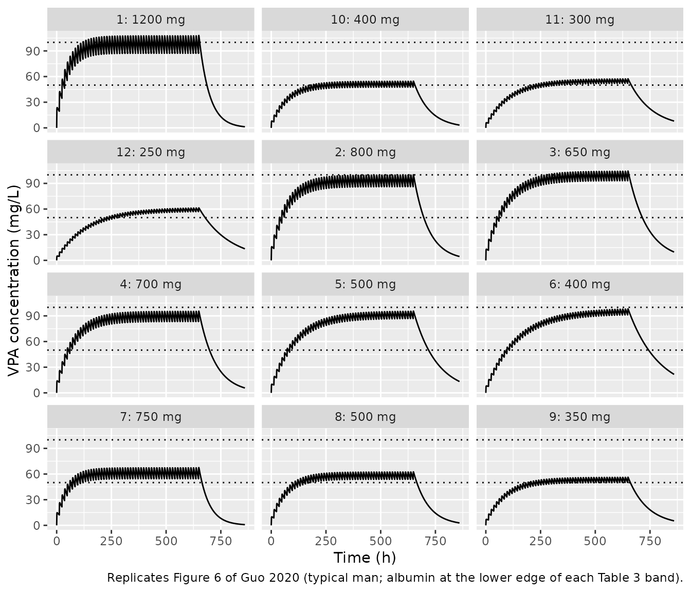
The top six panels are the high end of each Table 3 dose range and sit near the 100 mg/L upper target, as in the paper. The steady-state average concentration is a closed-form check on clearance alone:
cl_typ <- function(alb, nonem) 0.64 * (alb / 38.7)^-1.06 * exp(-0.45 * nonem)

fig6_ss <- sim_fig6 |>
  filter(time >= 648, time <= 660) |>
  group_by(panel, dose) |>
  summarise(
    trough = Cc[time == 648],
    peak = max(Cc),
    .groups = "drop"
  ) |>
  left_join(fig6 |> select(panel, ALB, CYP2C19_NON_EM), by = "panel") |>
  mutate(cavg_closed_form = dose / (tau * cl_typ(ALB, CYP2C19_NON_EM)))

fig6_ss |>
  dplyr::rename(
    "Panel" = panel, "Dose (mg BID)" = dose, "Albumin (g/L)" = ALB,
    "CYP2C19 non-EM" = CYP2C19_NON_EM, "Trough (mg/L)" = trough,
    "Peak (mg/L)" = peak, "Cavg = Dose/(tau CL) (mg/L)" = cavg_closed_form
  ) |>
knitr::kable(digits = 1)| Panel | Dose (mg BID) | Trough (mg/L) | Peak (mg/L) | Albumin (g/L) | CYP2C19 non-EM | Cavg = Dose/(tau CL) (mg/L) |
|---|---|---|---|---|---|---|
| 1 | 1200 | 87.2 | 108.1 | 25 | 0 | 98.3 |
| 2 | 800 | 86.1 | 100.1 | 35 | 0 | 93.6 |
| 3 | 650 | 93.1 | 104.5 | 45 | 0 | 99.3 |
| 4 | 700 | 83.4 | 95.6 | 25 | 1 | 90.0 |
| 5 | 500 | 86.9 | 95.6 | 35 | 1 | 91.8 |
| 6 | 400 | 91.2 | 98.2 | 45 | 1 | 95.8 |
| 7 | 750 | 54.5 | 67.5 | 25 | 0 | 61.5 |
| 8 | 500 | 53.8 | 62.5 | 35 | 0 | 58.5 |
| 9 | 350 | 50.1 | 56.2 | 45 | 0 | 53.5 |
| 10 | 400 | 47.6 | 54.6 | 25 | 1 | 51.4 |
| 11 | 300 | 52.1 | 57.4 | 35 | 1 | 55.1 |
| 12 | 250 | 57.0 | 61.4 | 45 | 1 | 59.9 |
top_row <- fig6_ss |> filter(panel <= 6)
stopifnot(
  # Figure 6 panels 1-6 plateau at about 95-100 mg/L. A sign error on
  # either clearance covariate moves at least one of these by > 50%.
  all(top_row$cavg_closed_form > 85 & top_row$cavg_closed_form < 105),
  # Male volume: the panel 1 swing is about 25 mg/L in Figure 6
  # (female volume would give about 45 mg/L).
  with(top_row[top_row$panel == 1, ], peak - trough > 18 & peak - trough < 32)
)
The bottom six panels (the low end of each Table 3 range) plateau at about 55-70 mg/L in Figure 6; evaluated at the same albumin edges the model gives 50-62 mg/L. The paper does not say which albumin value those panels used, so this 5-15% difference is not treated as a discrepancy.
PKNCA: steady-state exposure
PKNCA on the last dosing interval before washout (648-660 h) of the
Figure 6 simulation, compared with the closed-form steady-state
AUCtau = Dose / CL.
conc_ss <- sim_fig6 |>
  filter(!is.na(Cc), time >= 648, time <= 660) |>
  mutate(treatment = paste0("panel", panel)) |>
  select(id, time, Cc, treatment)

dose_ss <- ev_fig6 |>
  filter(evid == 1L, time == 648) |>
  left_join(fig6 |> select(id, panel), by = "id") |>
  mutate(treatment = paste0("panel", panel)) |>
  select(id, time, amt, treatment)

conc_obj <- PKNCAconc(conc_ss, Cc ~ time | treatment + id)
dose_obj <- PKNCAdose(dose_ss, amt ~ time | treatment + id)
intervals <- data.frame(
  start = 648, end = 660,
  cmax = TRUE, cmin = TRUE, auclast = TRUE, cav = TRUE
)
nca_res <- pk.nca(PKNCAdata(conc_obj, dose_obj, intervals = intervals))

ref_ss <- fig6_ss |>
  transmute(
    treatment = paste0("panel", panel),
    auclast = dose / cl_typ(ALB, CYP2C19_NON_EM),
    cav = cavg_closed_form
  )

cmp <- nlmixr2lib::ncaComparisonTable(
  simulated = nca_res,
  reference = ref_ss,
  by = "treatment",
  params = c("auclast", "cav"),
  units = c(auclast = "mg*h/L", cav = "mg/L"),
  tolerance_pct = 2
)
knitr::kable(
  cmp,
  caption = "Steady-state PKNCA vs. closed-form Dose/CL (typical patients of Figure 6). * differs by > 2%."
)| NCA parameter | treatment | Reference | Simulated | % diff |
|---|---|---|---|---|
| AUClast (mg*h/L) | panel1 | 1180 | 1180 | -0.0% |
| AUClast (mg*h/L) | panel2 | 1120 | 1120 | -0.0% |
| AUClast (mg*h/L) | panel3 | 1190 | 1190 | -0.1% |
| AUClast (mg*h/L) | panel4 | 1080 | 1080 | -0.0% |
| AUClast (mg*h/L) | panel5 | 1100 | 1100 | -0.2% |
| AUClast (mg*h/L) | panel6 | 1150 | 1140 | -0.9% |
| AUClast (mg*h/L) | panel7 | 737 | 737 | -0.0% |
| AUClast (mg*h/L) | panel8 | 702 | 702 | -0.0% |
| AUClast (mg*h/L) | panel9 | 642 | 641 | -0.1% |
| AUClast (mg*h/L) | panel10 | 617 | 617 | -0.0% |
| AUClast (mg*h/L) | panel11 | 661 | 659 | -0.2% |
| AUClast (mg*h/L) | panel12 | 719 | 713 | -0.9% |
| Cavg (mg/L) | panel1 | 98.3 | 98.3 | -0.0% |
| Cavg (mg/L) | panel2 | 93.6 | 93.6 | -0.0% |
| Cavg (mg/L) | panel3 | 99.3 | 99.2 | -0.1% |
| Cavg (mg/L) | panel4 | 90 | 89.9 | -0.0% |
| Cavg (mg/L) | panel5 | 91.8 | 91.6 | -0.2% |
| Cavg (mg/L) | panel6 | 95.8 | 95 | -0.9% |
| Cavg (mg/L) | panel7 | 61.5 | 61.4 | -0.0% |
| Cavg (mg/L) | panel8 | 58.5 | 58.5 | -0.0% |
| Cavg (mg/L) | panel9 | 53.5 | 53.4 | -0.1% |
| Cavg (mg/L) | panel10 | 51.4 | 51.4 | -0.0% |
| Cavg (mg/L) | panel11 | 55.1 | 55 | -0.2% |
| Cavg (mg/L) | panel12 | 59.9 | 59.4 | -0.9% |
nca_tab <- as.data.frame(nca_res) |>
  filter(PPTESTCD == "auclast") |>
  left_join(ref_ss, by = "treatment")
# Panels 6 and 12 (slowest elimination) are ~99% of the way to steady state
# at 648 h, so they sit ~1% below the closed form; 2% leaves headroom.
stopifnot(all(abs(nca_tab$PPORRES / nca_tab$auclast - 1) < 0.02))
Virtual cohort: oral and intravenous 500/400 mg twice daily
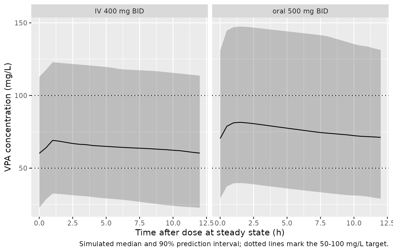
A stochastic cohort resembling Table 1: albumin drawn from a normal distribution (mean 38.9, SD 6.4 g/L) restricted to the observed 25.6-53.6 g/L range by redrawing, 24/60 CYP2C19 variant carriers and 16/60 women. Each patient receives the paper’s standard oral regimen (500 mg twice daily) or its intravenous regimen (400 mg twice daily, given here as a 1-h infusion; the paper does not state the infusion time).
rxode2::rxSetSeed(20200826)
n_per_arm <- 200

draw_alb <- function(n) {
  x <- rnorm(n, 38.9, 6.4)
  bad <- x < 25.6 | x > 53.6
  while (any(bad)) {
    x[bad] <- rnorm(sum(bad), 38.9, 6.4)
    bad <- x < 25.6 | x > 53.6
  }
  x
}

cohort <- tibble(
  id = seq_len(2 * n_per_arm),
  route = rep(c("oral 500 mg BID", "IV 400 mg BID"), each = n_per_arm),
  ALB = draw_alb(2 * n_per_arm),
  CYP2C19_NON_EM = rbinom(2 * n_per_arm, 1, 24 / 60),
  SEXF = rbinom(2 * n_per_arm, 1, 16 / 60)
)

n_dose_c <- 28 # two weeks, well past steady state for the slowest patients
dose_c <- cohort |>
  tidyr::crossing(k = seq_len(n_dose_c) - 1) |>
  mutate(
    time = k * 12,
    amt = ifelse(route == "oral 500 mg BID", 500, 400),
    cmt = ifelse(route == "oral 500 mg BID", "depot", "central"),
    rate = ifelse(route == "oral 500 mg BID", 0, 400),
    evid = 1L
  ) |>
  select(-k)
obs_c <- cohort |>
  tidyr::crossing(time = seq(312, 324, by = 0.5)) |>
  mutate(amt = 0, cmt = "central", rate = 0, evid = 0L)
ev_c <- bind_rows(dose_c, obs_c) |>
  arrange(id, time, desc(evid))

sim_c <- rxode2::rxSolve(
  mod, ev_c,
  keep = c("route", "CYP2C19_NON_EM", "SEXF", "ALB"),
  returnType = "data.frame"
)
sim_c |>
  filter(!is.na(Cc)) |>
  mutate(tad = time - 312) |>
  group_by(route, tad) |>
  summarise(
    q05 = quantile(Cc, 0.05), q50 = median(Cc), q95 = quantile(Cc, 0.95),
    .groups = "drop"
  ) |>
  ggplot(aes(tad, q50)) +
  geom_ribbon(aes(ymin = q05, ymax = q95), alpha = 0.25) +
  geom_line() +
  geom_hline(yintercept = c(50, 100), linetype = "dotted") +
  facet_wrap(~route) +
  labs(
    x = "Time after dose at steady state (h)", y = "VPA concentration (mg/L)",
    caption = "Simulated median and 90% prediction interval; dotted lines mark the 50-100 mg/L target."
  )
troughs <- sim_c |>
  filter(time == 324) |>
  mutate(genotype = ifelse(CYP2C19_NON_EM == 1, "variant carrier", "\\*1/\\*1"))

troughs |>
  group_by(route, genotype) |>
  summarise(
    n = n(),
    median = median(Cc),
    p05 = quantile(Cc, 0.05),
    p95 = quantile(Cc, 0.95),
    pct_50_100 = 100 * mean(Cc >= 50 & Cc <= 100),
    .groups = "drop"
  ) |>
  dplyr::rename(
    "Route" = route, "CYP2C19" = genotype, "N" = n,
    "Median trough (mg/L)" = median, "5th pct" = p05, "95th pct" = p95,
    "% within 50-100 mg/L" = pct_50_100
  ) |>
knitr::kable(digits = 1)| Route | CYP2C19 | N | Median trough (mg/L) | 5th pct | 95th pct | % within 50-100 mg/L |
|---|---|---|---|---|---|---|
| IV 400 mg BID | *1/*1 | 116 | 46.6 | 21.4 | 101.6 | 39.7 |
| IV 400 mg BID | variant carrier | 84 | 73.8 | 41.3 | 118.7 | 63.1 |
| oral 500 mg BID | *1/*1 | 119 | 59.0 | 26.8 | 119.9 | 43.7 |
| oral 500 mg BID | variant carrier | 81 | 88.9 | 46.6 | 155.4 | 59.3 |
Variant carriers have about 1.6-fold higher steady-state exposure
than *1/*1 patients at the same dose
(exp(0.45) = 1.57), which is why Table 3 of the paper
recommends roughly 40% lower doses for them.
ratio <- troughs |>
  filter(route == "oral 500 mg BID") |>
  group_by(CYP2C19_NON_EM) |>
  summarise(med = median(Cc), .groups = "drop")
ratio_nonem <- ratio$med[ratio$CYP2C19_NON_EM == 1] / ratio$med[ratio$CYP2C19_NON_EM == 0]
ratio_nonem
#> [1] 1.505239
# Centre-of-distribution check (robust to which subjects land in the tails):
# the genotype effect is exp(0.45) = 1.57 on average exposure; a sign error
# would put this ratio below 1.
stopifnot(ratio_nonem > 1.2, ratio_nonem < 2.1)
Assumptions and deviations
-
Signs of the covariate coefficients. The minus
signs on the albumin exponent (-1.06) and the CYP2C19 coefficient
(-0.45) are printed as a special glyph in the PDF that some text
extractors drop. The signs are confirmed by the printed 95% confidence
intervals (-1.87 to -0.26 and -0.66 to -0.25), by the Discussion
(clearance rises as albumin falls), and by Table 3 (higher doses for low
albumin and for
*1/*1patients). - Bioavailability. The paper pools oral and intravenous data with no bioavailability parameter, so oral bioavailability is taken as 1 and the estimated CL and V are systemic values.
-
IIV scale. Table 2 reports IIV as CV%. For
log-normal etas this was converted to variance as
log(1 + CV^2). The Results text quotes the final-model IIV on CL as 44.06%, while Table 2 gives 44.66%; the table value is used. - Residual error. Table 2 reports the proportional error as 11.75 with no unit; it is read as a percentage (proportional SD = 0.1175), which fits the less-than-5% assay CV and the sparse TDM design.
- Intravenous infusion time. Not reported; the virtual cohort uses a 1-h infusion for illustration. The model has no duration parameter, so users should supply the infusion rate that matches their regimen.
-
CYP2C19 grouping.
*17was genotyped but was not used to define the groups; only*2and*3carriers count as variant carriers (CYP2C19_NON_EM = 1). - Figure 6 inputs. The albumin values and sex used for Figure 6 are not printed. They were inferred from the figure itself (see above), and only the top row was used as a gate.
- Supplement. The online supplement (Table S1, literature summary; Table S2, stepwise covariate search) was checked. Its final step (V-GNDR, CL-CYP2C19, CL-ALB; objective function 817.623) matches the published final model and adds no parameter values.