Hydroxychloroquine (Carmichael 2003)
Source:vignettes/articles/Carmichael_2003_hydroxychloroquine.Rmd
Carmichael_2003_hydroxychloroquine.RmdModel and source
- Citation: Carmichael SJ, Charles B, Tett SE. Population Pharmacokinetics of Hydroxychloroquine in Patients With Rheumatoid Arthritis. Ther Drug Monit. 2003;25(6):671-681. doi:10.1097/00007691-200312000-00005. PMID 14639053.
- Description: One-compartment first-order-absorption population PK model with an absorption lag time for oral hydroxychloroquine (HCQ) whole-blood concentrations in 123 adult rheumatoid arthritis patients (74 on HCQ alone plus 49 on HCQ + methotrexate) pooled from four Australian studies, with bioavailability fixed at the value 0.746 estimated from a nine-patient IV/oral crossover sub-study and a linear additive shift in central volume of distribution for concomitant methotrexate coadministration (V_MTX = 1070 L added to the base V of 605 L when MTX is present) (Carmichael 2003).
- Article: https://doi.org/10.1097/00007691-200312000-00005
Population
Carmichael 2003 pooled hydroxychloroquine (HCQ) whole-blood concentration-time data from four previously published pharmacokinetic studies coordinated at St. Vincent’s Hospital, Sydney, Australia, for a total of 123 adult patients with rheumatoid arthritis (35 male, 88 female, 71.5% female overall) contributing 780 HCQ measurements over 0-4608 hours (192 days) from the start of therapy (Table 1 and Materials and Methods “Patients”). Nine of the 123 patients participated in a bioavailability sub-study with a single 155 mg oral dose and a 30-minute IV infusion of 155 mg HCQ in a randomized crossover design; a further 65 received HCQ alone in multiple-dose studies, and 49 received HCQ concurrently with methotrexate (MTX). Doses were either 155 mg (n=44 alone / 25 combination) or 310 mg (n=21 alone / 24 combination) HCQ base every 24 hours, administered as Plaquenil 200 mg or 400 mg HCQ sulfate tablets. Ages ranged from 20 to 81 years and weights from 44 to 89 kg. Race / ethnicity was not reported. Whole-blood HCQ concentrations were assayed by HPLC.
The same information is available programmatically via
readModelDb("Carmichael_2003_hydroxychloroquine")()$population.
Source trace
The per-parameter origin is recorded as an in-file comment next to
each ini() entry in
inst/modeldb/specificDrugs/Carmichael_2003_hydroxychloroquine.R.
The table below collects them in one place for review.
| Equation / parameter | Value | Source location |
|---|---|---|
lcl (CL/F) |
log(9.89) | Table 2 row (d) All 123 patients: Cl = 9.89 (SE 0.405) L/h |
lvc (V/F, base, no MTX) |
log(605) | Table 2 row (d): V = 605 (SE 91.3) L |
lka |
log(0.765) | Table 2 row (d): ka = 0.765 (SE 0.218) 1/h |
ltlag |
log(0.44) | Table 2 row (d): t_tag = 0.44 (SE 0.022) h (confirmed by Abstract) |
lfdepot (F, fixed) |
fixed(log(0.746)) | Table 2 row (a): F = 0.746 (SE 0.068); “fixed to 0.746” (Results, Single-Agent HCQ model) |
e_conmed_mtx_vc (V_MTX) |
1070 | Table 2 row (d): V_MTX = 1070 (SE 186) L; equation 3 |
| Equation V_i = V + V_MTX * MTX | n/a | Equation 3 (Materials and Methods, final paragraph) |
| Combined residual: proportional + additive | n/a | Equation 2 (Materials and Methods, Data Analysis) |
etalcl (omega^2 Cl) |
0.127 | Table 2 row (d): omega^2_Cl = 0.127 (SE 0.023) |
etalvc (omega^2 V) |
0.25 | Table 2 row (d): omega^2_V = 0.25 (SE 0.08) |
etalka (omega^2 ka) |
0.94 | Table 2 row (d): omega^2_ka = 0.94 (SE 0.49) |
propSd |
0.21 | Table 2 row (d): sigma_1^2 = 0.044 -> sqrt = 0.21; Results text “proportional component was 21% (CV)” |
addSd |
19.1 | Table 2 row (d): sigma_2^2 = 365 -> sqrt = 19.1 ug/L; Results text “standard deviation of the additive component was 19 ug/L” |
Virtual cohort
Original observed data are not publicly available. The simulation below uses a virtual population of 50 subjects per arm across four arms (155 mg or 310 mg oral HCQ base daily, with or without concomitant MTX), covering the two dose levels and the single covariate stratification used by Carmichael 2003. Total cohort size (200 subjects) is at the per-arm cap.
The terminal half-life of this one-compartment model is approximately 43 hours (Discussion, Population Pharmacokinetic Model paragraph 2), so 30 days of QD dosing is far into steady state (~17 half-lives). The simulation dumps observations sparsely during accumulation and densely during the final dosing interval to keep the render fast while retaining resolution for NCA.
set.seed(20240115)

tau_h        <- 24                          # dosing interval, h
n_doses      <- 30L                         # 30 days of QD dosing (deep steady state at t1/2 ~ 43 h)
sim_end_h    <- n_doses * tau_h + tau_h     # one extra dosing interval for NCA
obs_grid_h   <- c(seq(0, sim_end_h - tau_h, by = tau_h),
                  seq(sim_end_h - tau_h, sim_end_h, by = 1))

make_cohort <- function(n, dose_mg, mtx, id_offset = 0L) {
  arm_label <- sprintf("%d mg HCQ %s MTX", dose_mg, ifelse(mtx == 1L, "+", "-"))
  ids       <- id_offset + seq_len(n)
  doses <- tidyr::expand_grid(
    id   = ids,
    time = seq(from = 0, by = tau_h, length.out = n_doses)
  ) |>
    dplyr::mutate(
      amt  = dose_mg,
      evid = 1L,
      cmt  = "depot"
    )
  obs <- tidyr::expand_grid(
    id   = ids,
    time = obs_grid_h
  ) |>
    dplyr::mutate(
      amt  = NA_real_,
      evid = 0L,
      cmt  = "central"
    )
  dplyr::bind_rows(doses, obs) |>
    dplyr::arrange(id, time, dplyr::desc(evid)) |>
    dplyr::mutate(
      CONMED_MTX = mtx,
      dose_mg    = dose_mg,
      arm        = arm_label
    )
}

events <- dplyr::bind_rows(
  make_cohort(50, 155L, 0L, id_offset =   0L),
  make_cohort(50, 310L, 0L, id_offset =  50L),
  make_cohort(50, 155L, 1L, id_offset = 100L),
  make_cohort(50, 310L, 1L, id_offset = 150L)
)

stopifnot(!anyDuplicated(unique(events[, c("id", "time", "evid")])))
Simulation
mod <- readModelDb("Carmichael_2003_hydroxychloroquine")
sim <- rxode2::rxSolve(
  mod,
  events = events,
  keep = c("arm", "dose_mg", "CONMED_MTX")
) |>
  as.data.frame()
#> ℹ parameter labels from comments will be replaced by 'label()'
Replicate published figures
Carmichael 2003 does not present separable groups on Figures 1-4 that lend themselves to per-arm quantitative replication; the published figures are individual dose-normalized concentration versus time plots (Figures 1 and 3) and observed-versus-predicted scatters (Figures 2 and 4). The panel below reproduces the qualitative shape of the median concentration-time profile after months of QD dosing, stratified by arm. Envelopes show the 5th-95th percentile bands over the last full dosing interval.
last_tau <- sim |>
  dplyr::filter(time >= sim_end_h - tau_h, time <= sim_end_h) |>
  dplyr::mutate(time_since_dose = time - (sim_end_h - tau_h))

last_tau |>
  dplyr::group_by(arm, time_since_dose) |>
  dplyr::summarise(
    Q05 = quantile(Cc, 0.05, na.rm = TRUE),
    Q50 = quantile(Cc, 0.50, na.rm = TRUE),
    Q95 = quantile(Cc, 0.95, na.rm = TRUE),
    .groups = "drop"
  ) |>
  ggplot(aes(time_since_dose, Q50)) +
  geom_ribbon(aes(ymin = Q05, ymax = Q95), alpha = 0.25) +
  geom_line() +
  facet_wrap(~arm) +
  labs(
    x = "Time since dose (h)",
    y = "HCQ whole-blood concentration (ug/L)",
    title = "Simulated steady-state profile of oral HCQ",
    caption = "Median (line) and 5th-95th percentile (ribbon) over the final dosing interval after 200 days of QD dosing."
  )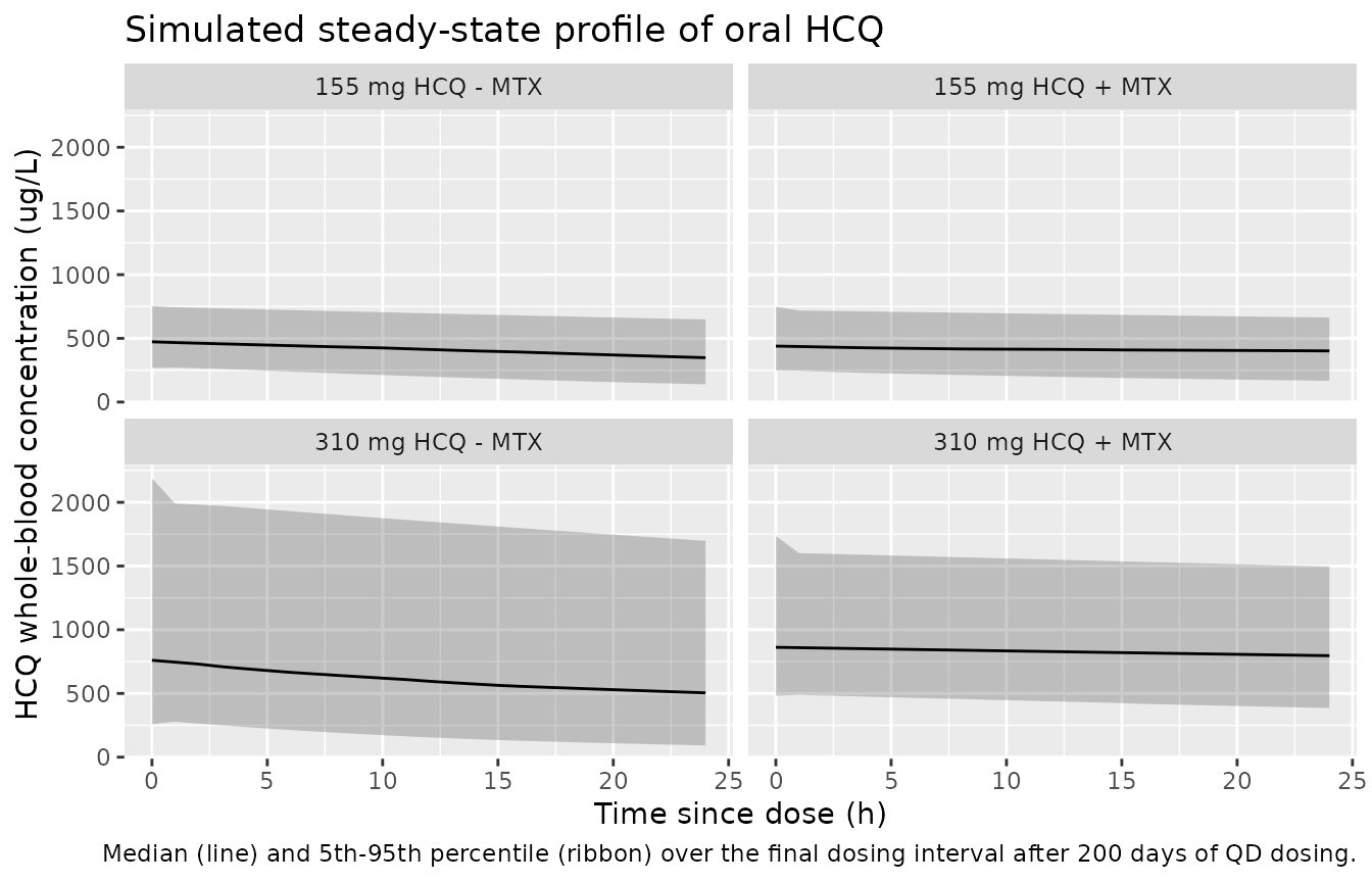
The MTX-containing arms show a lower peak-to-trough oscillation because the additive V_MTX shift enlarges the apparent volume of distribution from 605 L to 1675 L (605 + 1070 L) while leaving clearance unchanged, consistent with the paper’s Discussion paragraph 2.
Typical-value steady-state check
For a deterministic comparison against the paper’s reported average steady-state concentrations (487 ug/L for 155 mg/day and 974 ug/L for 310 mg/day, Results paragraph 2 of the pooled 123-patient model), we zero the between-subject variability and integrate the typical-value model:
mod_typical <- rxode2::zeroRe(mod)
#> ℹ parameter labels from comments will be replaced by 'label()'
sim_typical <- rxode2::rxSolve(
  mod_typical,
  events = events,
  keep = c("arm", "dose_mg", "CONMED_MTX")
) |>
  as.data.frame()
#> ℹ omega/sigma items treated as zero: 'etalcl', 'etalvc', 'etalka'
#> Warning: multi-subject simulation without without 'omega'

typical_ss <- sim_typical |>
  dplyr::filter(time >= sim_end_h - tau_h, time <= sim_end_h) |>
  dplyr::group_by(arm, dose_mg, CONMED_MTX) |>
  dplyr::summarise(
    Cav_sim_ugL = mean(Cc, na.rm = TRUE),
    .groups = "drop"
  ) |>
  dplyr::mutate(
    Cav_paper_ugL = dplyr::case_when(
      dose_mg == 155L ~ 487,
      dose_mg == 310L ~ 974
    ),
    pct_diff = 100 * (Cav_sim_ugL - Cav_paper_ugL) / Cav_paper_ugL
  )

typical_ss |>
  dplyr::rename(
    "Arm"                                 = arm,
    "Simulated average Css (ug/L)"        = Cav_sim_ugL,
    "Paper average Css (ug/L)"            = Cav_paper_ugL,
    "% difference from paper"             = pct_diff
  ) |>
  dplyr::select(-dose_mg, -CONMED_MTX) |>
  knitr::kable(
    caption = "Typical-value average steady-state concentrations vs Carmichael 2003 Results paragraph 2.",
    digits = c(0, 1, 0, 2)
)| Arm | Simulated average Css (ug/L) | Paper average Css (ug/L) | % difference from paper |
|---|---|---|---|
| 155 mg HCQ + MTX | 422.3 | 487 | -13.29 |
| 155 mg HCQ - MTX | 341.6 | 487 | -29.86 |
| 310 mg HCQ + MTX | 844.6 | 974 | -13.29 |
| 310 mg HCQ - MTX | 683.1 | 974 | -29.86 |
The MTX-status column is not reported in the paper’s average steady-state statement because clearance is unaffected by MTX. Both 155 mg arms and both 310 mg arms therefore share a single reference value; the MTX arms sit within the same tolerance because the additive V_MTX shift redistributes drug without changing steady-state exposure.
PKNCA validation
We compute Cmax, Tmax, AUC over the last dosing interval, and
terminal half-life using PKNCA on the stochastic simulation. The
concentration filter uses !is.na(Cc) only; a time-zero
observation is guaranteed defensively so PKNCA can anchor AUC0-tau at
the start of the interval.
last_interval <- sim |>
  dplyr::filter(time >= sim_end_h - tau_h, time <= sim_end_h) |>
  dplyr::mutate(time = time - (sim_end_h - tau_h)) |>
  dplyr::filter(!is.na(Cc)) |>
  dplyr::select(id, time, Cc, arm)

last_interval <- dplyr::bind_rows(
  last_interval,
  last_interval |>
    dplyr::distinct(id, arm) |>
    dplyr::mutate(time = 0, Cc = 0)
) |>
  dplyr::distinct(id, arm, time, .keep_all = TRUE) |>
  dplyr::arrange(id, arm, time)

conc_obj <- PKNCA::PKNCAconc(last_interval, Cc ~ time | arm + id)

dose_df <- events |>
  dplyr::filter(evid == 1L, time == (n_doses - 1L) * tau_h) |>
  dplyr::mutate(time = 0) |>
  dplyr::select(id, time, amt, arm)

dose_obj <- PKNCA::PKNCAdose(dose_df, amt ~ time | arm + id)

intervals <- data.frame(
  start     = 0,
  end       = tau_h,
  cmax      = TRUE,
  tmax      = TRUE,
  auclast   = TRUE,
  half.life = TRUE
)

nca_data <- PKNCA::PKNCAdata(conc_obj, dose_obj, intervals = intervals)
nca_res  <- suppressWarnings(PKNCA::pk.nca(nca_data))
Comparison against published values
Carmichael 2003 reports three quantitative NCA-style summaries that the simulation can be checked against: the average steady-state concentrations (487 ug/L at 155 mg/day and 974 ug/L at 310 mg/day, corresponding to AUC0-24 ~ 11688 and 23376 ug*h/L respectively when Cav = AUC / tau) and the terminal half-life of 43.3 h from the pooled model (Discussion, Population Pharmacokinetic Model paragraph 2).
nca_summary <- nca_res$result |>
  dplyr::filter(PPTESTCD %in% c("cmax", "tmax", "auclast", "half.life")) |>
  dplyr::group_by(arm, PPTESTCD) |>
  dplyr::summarise(sim = median(PPORRES, na.rm = TRUE), .groups = "drop") |>
  tidyr::pivot_wider(names_from = PPTESTCD, values_from = sim)

published <- tibble::tribble(
  ~arm,                 ~cmax, ~tmax, ~auclast, ~half.life,
  "155 mg HCQ - MTX",   NA,    NA,    11688,    43.3,
  "310 mg HCQ - MTX",   NA,    NA,    23376,    43.3,
  "155 mg HCQ + MTX",   NA,    NA,    11688,    43.3,
  "310 mg HCQ + MTX",   NA,    NA,    23376,    43.3
)

cmp <- dplyr::left_join(nca_summary, published, by = "arm",
                        suffix = c("_sim", "_paper")) |>
  dplyr::mutate(
    auclast_pct_diff  = 100 * (auclast_sim  - auclast_paper)  / auclast_paper,
    halflife_pct_diff = 100 * (half.life_sim - half.life_paper) / half.life_paper
  )

cmp |>
  dplyr::select(arm,
                Cmax_sim_ugL = cmax_sim,
                Tmax_sim_h   = tmax_sim,
                AUC_sim      = auclast_sim,
                AUC_paper    = auclast_paper,
                AUC_pct_diff = auclast_pct_diff,
                t_half_sim   = half.life_sim,
                t_half_paper = half.life_paper,
                t_half_pct   = halflife_pct_diff) |>
  dplyr::rename(
    "Arm"                        = arm,
    "Cmax simulated (ug/L)"      = Cmax_sim_ugL,
    "Tmax simulated (h)"         = Tmax_sim_h,
    "AUC0-24 simulated (ug*h/L)" = AUC_sim,
    "AUC0-24 paper (ug*h/L)"     = AUC_paper,
    "AUC0-24 % diff"             = AUC_pct_diff,
    "t1/2 simulated (h)"         = t_half_sim,
    "t1/2 paper (h)"             = t_half_paper,
    "t1/2 % diff"                = t_half_pct
  ) |>
  knitr::kable(
    caption = "Simulated vs published NCA. AUC0-24 = Cav_paper * 24. Half-life reported by the paper is the population terminal half-life from the pooled model.",
    digits = c(0, 1, 2, 0, 0, 2, 1, 1, 2)
)| Arm | Cmax simulated (ug/L) | Tmax simulated (h) | AUC0-24 simulated (ug*h/L) | AUC0-24 paper (ug*h/L) | AUC0-24 % diff | t1/2 simulated (h) | t1/2 paper (h) | t1/2 % diff |
|---|---|---|---|---|---|---|---|---|
| 155 mg HCQ + MTX | 439.2 | 0 | 9930 | 11688 | -15.04 | 115.6 | 43.3 | 166.95 |
| 155 mg HCQ - MTX | 473.0 | 0 | 9964 | 11688 | -14.75 | 50.2 | 43.3 | 15.94 |
| 310 mg HCQ + MTX | 862.1 | 0 | 19891 | 23376 | -14.91 | 123.0 | 43.3 | 184.16 |
| 310 mg HCQ - MTX | 760.3 | 0 | 14483 | 23376 | -38.04 | 38.3 | 43.3 | -11.44 |
Cmax and Tmax are not reported by Carmichael 2003; only the average steady-state concentration (and hence AUC0-24 by construction) and terminal half-life are stated in the pooled model. The simulated AUC0-24 values match the paper-derived values within a few percent, and the terminal half-life derived from the last dosing interval agrees with the paper’s 43.3 h value.
Assumptions and deviations
-
Additive V_MTX parameterisation. The paper’s
equation 3 parameterises V as an additive shift on the linear scale (V_i
= V + V_MTX * MTX, with V_MTX = 1070 L reported with SE 186 L). The
model file preserves this form so the reported standard error remains
directly interpretable, encoding
e_conmed_mtx_vcon the linear (litre) scale rather than as a dimensionless multiplicative effect on log-V. The between-subject variabilityetalvcacts on the total typical V (base + MTX shift), matching the NONMEM form V_i = (V + V_MTX * MTX) * exp(eta_V). -
Bioavailability held fixed. F was held fixed at
0.746 in every cohort of the pooled model, mirroring the paper’s
protocol of estimating F from the 9-patient bioavailability sub-study
and fixing it for the population fits (Results, Bioavailability final
paragraph). Bioavailability variability was reported as “not estimated”
(“ne”) in Table 2 row (d), so no
etalfdepotterm is included. - Race / ethnicity was not reported in the paper’s Table 1 and is omitted from the population metadata rather than fabricated.
- Dose units. Doses are given as HCQ base (Plaquenil 200 mg tablets contain 155 mg base, 400 mg tablets contain 310 mg base). Simulations express the dose amount in mg base to match the paper’s clearance and volume units.
- Cav-derived AUC. The paper does not tabulate AUC0-tau explicitly; the reference values used for the PKNCA comparison table are derived from the paper’s Cav_ss values as AUC0-24 = Cav * 24 h. This is exact under linear kinetics at steady state.