Ivermectin (Fimbo 2023)
Source:vignettes/articles/Fimbo_2023_ivermectin.Rmd
Fimbo_2023_ivermectin.RmdModel and source
Citation: Fimbo AM, Mlugu EM, Kitabi EN, Kulwa GS, Iwodyah MA, Mnkugwe RH, Kunambi PP, Malishee A, Kamuhabwa AAR, Minzi OM, Aklillu E (2023). Population pharmacokinetics of ivermectin after mass drug administration in lymphatic filariasis endemic communities of Tanzania. CPT Pharmacometrics Syst Pharmacol 12(12):1884-1896. doi:10.1002/psp4.13038. Structural model adapted, via the NONMEM PRIOR subroutine, from Duthaler U et al. (2019) Br J Clin Pharmacol 85(3):626-633; all parameter values encoded here are Fimbo 2023’s own final estimates (Table 2), not Duthaler’s priors.
Description: Two-compartment population PK model for oral ivermectin (IVM) in 468 individuals aged 5-78 years and weighing more than 15 kg who received a single height-based IVM dose (3, 6, 9, or 12 mg) together with albendazole 400 mg during a lymphatic filariasis mass drug administration (MDA) campaign in the Mkinga district, Tanga region, Tanzania (1404 plasma samples drawn predose and at 2, 4, and 6 h). Absorption is the Savic analytical transit chain: a gamma-distributed input with mean transit time MTT = 1.523 h through NN = 6 transit compartments (fixed) feeds an absorption compartment that empties into the central compartment at ka = 0.708 /h. Body weight enters as allometric scaling with exponents fixed at 0.75 on CL/F and 1 on Vc/F, referenced to 70 kg; intercompartmental clearance Q/F and peripheral volume Vp/F are NOT allometrically scaled, which is what makes the model’s terminal half-life fall with increasing body weight (66 h in the 3 mg pool vs 38 h in the 12 mg pool). Dose group is the only retained covariate: relative bioavailability is 48.2% higher in the 3 mg dose pool than in the 6, 9, and 12 mg pools. A two-class NONMEM mixture on MTT identifies a 16.1% subpopulation whose mean transit time is 97.0% longer than the rest of the population; it is supplied here as the per-subject binary MIX_LONG_MTT. Sex, age, renal and hepatic laboratory markers and ABCB1 / CYP3A4 / CYP3A5 / CYP2C9 / CYP2C19 / CYP2J2 genotypes were screened and none were retained. Inter-individual variability is estimated on CL/F, Vc/F, Q/F, Vp/F, MTT and F (none on ka, which NONMEM fixed to zero); residual variability is purely proportional (26.2%), the additive term having been fixed to zero.
Article: https://doi.org/10.1002/psp4.13038
Supplement: https://www.ncbi.nlm.nih.gov/pmc/articles/PMC10725270/ Data S1 holds Figures S1-S3, Data S2 holds Tables S1-S3, and Data S3 holds the final NONMEM control stream. Note that the paper’s Methods misdirects here – it says “model code is presented in Data S1”, but the model code is in Data S3; Data S1 contains only the supplementary figures.
Fimbo 2023 fitted a two-compartment model with Savic transit absorption to 1404 ivermectin plasma samples from 468 people dosed during a lymphatic filariasis mass drug administration (MDA) campaign in the Mkinga district of Tanga region, Tanzania. Dose was assigned by height pole (3, 6, 9, or 12 mg), which the paper’s second contribution shows systematically underdoses heavier adults relative to weight-based dosing.
Population
| Field | Value |
|---|---|
| species | human |
| n_subjects | 468 |
| n_studies | 1 |
| n_observations | 1404 |
| age_range | 5-78 years |
| weight_range | roughly 15-90 kg (individuals below 15 kg are excluded from the MDA programme) |
| sex_female_pct | 40.1 |
| race_ethnicity | Black 100 |
| disease_state | MDA-eligible residents of lymphatic filariasis endemic communities; participants were prescreened for circulating filarial antigen and microfilaraemia but were treated regardless of infection status, so the cohort is the general at-risk population rather than a confirmed-infected one. Pregnant women and children under 5 years were excluded. |
| dose_range | single oral ivermectin 3, 6, 9, or 12 mg assigned by height pole (90-119, 119-139, 139-159, and >159 cm respectively; roughly 150-200 ug/kg), co-administered with albendazole 400 mg |
| regions | Mkinga district, Tanga region, north-eastern Tanzania |
| notes | Baseline demographic, clinical and biochemical characteristics are in Fimbo 2023 Table 1, stratified by dose pool (3 mg n = 12, 6 mg n = 49, 9 mg n = 159, 12 mg n = 248); genotype characteristics are in Table S2. Sex was recorded for 466 of 468 subjects (279 male, 187 female); the 40.1% female figure is 187/466. Weight and dose pool are strongly confounded because dosing was by height pole. NOTE: Fimbo 2023 Methods states participants were ‘aged between 5- and 78 years old’, but the per-weight-band age ranges in Table S1 extend to 91 years; the Methods range is recorded here and the discrepancy is flagged in the validation vignette. |
A total of 468 MDA-eligible individuals aged 5-78 years and weighing more than 15 kg were enrolled (Fimbo 2023 Table 1). Sex was recorded for 466: 279 male (59.9%) and 187 female (40.1%). Because dose is assigned by height pole, the dose pools are also weight and age strata, and the two are strongly confounded by construction:
| Dose pool | Dose (mg) | n | Weight mean (kg) | Weight SD (kg) | Age mean (years) | Height pole (cm) |
|---|---|---|---|---|---|---|
| 3 mg | 3 | 12 | 19.92 | 3.28 | 6.42 | 90-119 |
| 6 mg | 6 | 49 | 25.32 | 3.97 | 10.92 | 119-139 |
| 9 mg | 9 | 159 | 52.26 | 15.17 | 36.77 | 139-159 |
| 12 mg | 12 | 248 | 61.73 | 10.79 | 39.98 | >159 |
The genotype panel (ABCB1 c.3435C>T, ABCB1 rs3842, CYP2C19,
CYP2C9, CYP2J2, CYP3A4 *1B, CYP3A5) is in Fimbo 2023 Table S2; none of
these was retained (Table S3 runs 16-19). They are recorded in the model
file’s covariatesDataExcluded list for provenance.
Source trace
Every value below is also carried as an in-file comment beside its
ini() entry in
inst/modeldb/specificDrugs/Fimbo_2023_ivermectin.R.
| Equation / parameter | Value | Source location |
|---|---|---|
lcl (CL/F at 70 kg) |
7.698 L/h | Table 2, row “CL (L/h)”, RSE 7% |
lvc (Vc/F at 70 kg) |
146.1 L | Table 2, row “Vc (L)”, RSE 11% |
lq (Q/F) |
20.42 L/h | Table 2, row “Q (L/h)”, RSE 12% |
lvp (Vp/F) |
207.1 L | Table 2, row “Vp (L)”, RSE 11% |
lmtt (MTT) |
1.523 h | Table 2, row “MTT (h)”, RSE 5% |
lka (ka) |
0.7082 /h | Table 2, row “K a (/h)”, RSE 17% |
nn_fix (NN) |
6 (fixed) | Table 2, row “NN” = “6 (Fixed to this value)”; Data S3
$THETA (6) FIX
|
lfdepot (reference F) |
1 (fixed) | Results: “F1 was fixed to 1”; Data S3
TVBIO = 1 * (1 + THETA(10))**DOSE3MG
|
e_wt_cl |
0.75 (fixed) | Results equation CLi = CLpop x (WT/70)^0.75; Data S3
TVCL = THETA(1) * (WT/70)**0.75
|
e_wt_vc |
1 (fixed) | Results equation Vci = Vcpop x (WT/70); Data S3
TVV2 = THETA(2) * (WT/70)
|
e_dose_3mg_fdepot |
0.4822 | Table 2, “Proportional increase in bioavailability for the 3 mg dose”, RSE 40% |
e_mix_long_mtt_mtt |
0.9695 | Table 2, “Proportional difference in MTT between the subpopulation and the rest”, RSE 12% |
| Mixture fraction P(long MTT) | 0.1606 | Table 2, “Proportion of a subpopulation with a different typical
MTT”, RSE 30% (carried in covariateData, not
ini(), because it is a simulation input rather than a model
parameter) |
etalcl |
0.4458^2 | Table 2, “Interindividual variability for CL (%CV)” |
etalvc |
0.3339^2 | Table 2, “Interindividual variability for Vc (%CV)” |
etalq |
0.4856^2 | Table 2, “Interindividual variability for Q (%CV)” |
etalvp |
0.4125^2 | Table 2, “Interindividual variability for Vp (%CV)” |
etalmtt |
0.2589^2 | Table 2, “Interindividual variability for MTT (%CV)” |
etalfdepot |
0.278^2 | Table 2, “Interindividual variability for F (%CV)” |
| IIV on ka | none | Data S3 $OMEGA BLOCK(1) 0 FIX ; EKA
|
propSd |
0.262 | Table 2, “Proportional residual error”, RSE 3% |
| Additive residual error | absent | Data S3 $THETA (0) FIX ; ADD
|
d/dt(depot) <- transit(nn, mtt, fdepot) - ka * depot |
n/a | Data S3 $DES line 1 (analytical Savic chain with
KTR = (NN+1)/MTT, LNFAC = log(6!)) |
f(depot) <- 0 |
n/a | Data S3 $PK line F1 = 0, commented
“;;Prevent NONMEM from administering dose into absorption compartment as
this will be done through transit compartments” |
Cc <- 1000 * central / vc |
n/a | Data S3 S2 = V2/1000 ; dose in mg, DV in ng/mL
|
Two readings the supplement settled
Two values in Table 2 are ambiguous from the main text alone, and the Data S3 control stream resolves both. Recording them here because getting either wrong changes the model materially.
The IIV column is omega, not
%CV. Table 2 labels its variability rows
“Interindividual variability for CL (%CV)” with the footnote
“Inter-individual variabilities are on a standard deviation scale
(%CV)”, while the Methods define
CV% = 100 * sqrt(exp(omega^2) - 1). Those two readings
differ (for CL, omega = 0.4458 versus
CV = 0.4689). Data S3 decides it: the control stream’s
$OMEGA initial estimates are exactly the
squares of the corresponding Table S3
run10 entries.
| Parameter | Data S3 OMEGA) | ||
|---|---|---|---|
| CL | 0.2010 | 0.4479 | 0.4483 |
| Vc | 0.0758 | 0.2753 | 0.2753 |
| Q | 0.2470 | 0.4971 | 0.4970 |
| Vp | 0.1720 | 0.4147 | 0.4147 |
| MTT | 0.1600 | 0.4002 | 0.4000 |
| F | 0.0922 | 0.3036 | 0.3036 |
The residual error is purely proportional. Table 2
lists only a proportional term, and Data S3 confirms the additive term
was fixed out: $THETA (0) FIX ; ADD, entering
W = SQRT(ADD**2 + PROP**2*IPRED**2).
Structural checks
Two closed-form identities that must hold for a linear two-compartment model, independent of any published number. These compare the solver against algebra, so the difference is pure numerical error and a tight bound is appropriate.
mod <- readModelDb("Fimbo_2023_ivermectin")

# Linear-trapezoidal AUC over whatever grid is supplied. Sorts defensively so
# the result never depends on incoming row order.
trapz <- function(time, conc) {
  o <- order(time); time <- time[o]; conc <- conc[o]
  sum(diff(time) * (head(conc, -1) + tail(conc, -1)) / 2)
}

# Analytic terminal (beta) half-life of a 2-compartment model.
beta_half_life <- function(cl, vc, q, vp) {
  kel <- cl / vc; k12 <- q / vc; k21 <- q / vp
  b <- kel + k12 + k21
  beta <- 0.5 * (b - sqrt(b^2 - 4 * kel * k21))
  log(2) / beta
}

# Typical (population) parameters at a given weight, per the model equations.
typ_par <- function(wt) {
  list(cl = 7.698 * (wt / 70)^0.75,
       vc = 146.1 * (wt / 70),
       q  = 20.42,
       vp = 207.1)
}
# One typical individual per dose pool, at that pool's mean body weight,
# assigned to the reference (majority) MTT subpopulation. zeroRe() removes all
# IIV, so this simulation is fully deterministic and reproducible in CI.
grid_t <- c(seq(0, 12, by = 0.1), seq(12.5, 72, by = 0.5))

ev_typ <- dplyr::bind_rows(lapply(seq_len(nrow(dose_pools)), function(i) {
  p <- dose_pools[i, ]
  dose_row <- tibble::tibble(
    id = i, time = 0, amt = p$dose_mg, evid = 1L, cmt = "depot"
  )
  obs_rows <- tibble::tibble(
    id = i, time = grid_t, amt = NA_real_, evid = 0L, cmt = "central"
  )
  dplyr::bind_rows(dose_row, obs_rows) |>
    dplyr::mutate(
      pool         = p$pool,
      WT           = p$wt_mean,
      DOSE_3MG     = as.integer(p$dose_mg == 3),
      MIX_LONG_MTT = 0L
    )
})) |>
  dplyr::arrange(id, time, dplyr::desc(evid))

stopifnot(!anyDuplicated(unique(ev_typ[, c("id", "time", "evid")])))

sim_typ <- rxode2::rxSolve(
  rxode2::zeroRe(mod), events = ev_typ,
  keep = c("pool", "WT", "DOSE_3MG")
) |>
  as.data.frame()
#> ℹ omega/sigma items treated as zero: 'etalcl', 'etalvc', 'etalq', 'etalvp', 'etalmtt', 'etalfdepot'
#> Warning: multi-subject simulation without without 'omega'

stopifnot(all(sim_typ$Cc >= 0), !anyNA(sim_typ$Cc))
# PKNCA on the deterministic typical-value profiles.
nca_typ_in <- sim_typ |>
  dplyr::filter(!is.na(Cc)) |>
  dplyr::select(id, time, Cc, pool)

nca_typ_in <- dplyr::bind_rows(
  nca_typ_in,
  nca_typ_in |> dplyr::distinct(id, pool) |> dplyr::mutate(time = 0, Cc = 0)
) |>
  dplyr::distinct(id, pool, time, .keep_all = TRUE) |>
  dplyr::arrange(id, pool, time)

dose_typ <- ev_typ |>
  dplyr::filter(evid == 1L) |>
  dplyr::select(id, time, amt, pool)

nca_typ <- PKNCA::pk.nca(PKNCA::PKNCAdata(
  PKNCA::PKNCAconc(nca_typ_in, Cc ~ time | pool + id),
  PKNCA::PKNCAdose(dose_typ, amt ~ time | pool + id, route = "extravascular"),
  intervals = data.frame(start = 0, end = Inf,
                         cmax = TRUE, tmax = TRUE,
                         auclast = TRUE, aucinf.obs = TRUE, half.life = TRUE)
))

typ_wide <- as.data.frame(nca_typ) |>
  dplyr::select(pool, PPTESTCD, PPORRES) |>
  tidyr::pivot_wider(names_from = PPTESTCD, values_from = PPORRES)

# Identity 1: AUC(0-inf) must equal 1000 * F * Dose / CL exactly, because the
# model is linear. F = 1.4822 in the 3 mg pool and 1 elsewhere.
# Identity 2: PKNCA's terminal half-life must equal the analytic beta half-life.
ident <- dose_pools |>
  dplyr::left_join(typ_wide, by = "pool") |>
  dplyr::rowwise() |>
  dplyr::mutate(
    fbio        = if (dose_mg == 3) 1.4822 else 1,
    cl_i        = typ_par(wt_mean)$cl,
    auc_closed  = 1000 * fbio * dose_mg / cl_i,
    thalf_closed = do.call(beta_half_life, typ_par(wt_mean)),
    auc_pct     = 100 * (aucinf.obs - auc_closed) / auc_closed,
    thalf_pct   = 100 * (half.life - thalf_closed) / thalf_closed
  ) |>
  dplyr::ungroup()

ident |>
  dplyr::transmute(
    "Dose pool"                 = pool,
    "AUC0-inf, PKNCA"           = round(aucinf.obs, 1),
    "AUC0-inf, F*Dose/CL"       = round(auc_closed, 1),
    "AUC diff (%)"              = round(auc_pct, 3),
    "t1/2, PKNCA"               = round(half.life, 2),
    "t1/2, analytic beta"       = round(thalf_closed, 2),
    "t1/2 diff (%)"             = round(thalf_pct, 3)
  ) |>
knitr::kable(caption = "Solver vs closed form. Both differences are numerical error only.")| Dose pool | AUC0-inf, PKNCA | AUC0-inf, F*Dose/CL | AUC diff (%) | t1/2, PKNCA | t1/2, analytic beta | t1/2 diff (%) |
|---|---|---|---|---|---|---|
| 3 mg | 1480.0 | 1482.5 | -0.175 | 63.17 | 63.43 | -0.411 |
| 6 mg | 1668.0 | 1671.1 | -0.183 | 55.66 | 55.93 | -0.482 |
| 9 mg | 1453.1 | 1455.7 | -0.175 | 40.08 | 40.35 | -0.662 |
| 12 mg | 1710.1 | 1713.0 | -0.171 | 37.64 | 37.91 | -0.701 |
# Deterministic quantities: a tight bound is correct here and will go red on
# any structural mis-transcription (a wrong volume, exponent or unit factor).
stopifnot(
  max(abs(ident$auc_pct))   < 1.0,
  max(abs(ident$thalf_pct)) < 2.0
)
The AUC0-inf = 1000 * F * Dose / CL identity passing at
this tolerance is a strong joint check on the allometric exponent on
CL/F, the 3 mg bioavailability term, the f(depot) <- 0
suppression (if the dose bolus were not suppressed, the depot would
receive the dose twice and AUC would double), and the
1000 * mg/L to ng/mL conversion.
Comparison against published NCA
Fimbo 2023 Table 3 reports observed and model-estimated secondary PK
parameters per dose pool. The model-estimated column is the comparison
target; it is the column that also carries AUC0-inf and
terminal half-life, which cannot be computed from the observed data
(sampling stopped at 6 h).
published <- tibble::tribble(
  ~pool,  ~cmax, ~tmax, ~auclast, ~aucinf.obs, ~half.life,
  "3 mg",    41,   3.5,      147,        1534,         66,
  "6 mg",    50,   4.0,      171,        1770,         58,
  "9 mg",    49,   4.5,      169,        1521,         41,
  "12 mg",   54,   4.5,      190,        1681,         38
)

# Table 3's AUC0-6 is a 0-6 h partial area; recompute it on that window rather
# than reusing auclast (which runs to 72 h here).
nca_06 <- PKNCA::pk.nca(PKNCA::PKNCAdata(
  PKNCA::PKNCAconc(nca_typ_in, Cc ~ time | pool + id),
  PKNCA::PKNCAdose(dose_typ, amt ~ time | pool + id, route = "extravascular"),
  intervals = data.frame(start = 0, end = 6, auclast = TRUE)
))

simulated <- typ_wide |>
  dplyr::select(pool, cmax, tmax, aucinf.obs, half.life) |>
  dplyr::left_join(
    as.data.frame(nca_06) |>
      dplyr::filter(PPTESTCD == "auclast") |>
      dplyr::select(pool, auclast = PPORRES),
    by = "pool"
  )

cmp <- simulated |>
  tidyr::pivot_longer(-pool, names_to = "PPTESTCD", values_to = "Simulated") |>
  dplyr::left_join(
    published |> tidyr::pivot_longer(-pool, names_to = "PPTESTCD",
                                     values_to = "Published"),
    by = c("pool", "PPTESTCD")
  ) |>
  dplyr::mutate(
    pct_diff = 100 * (Simulated - Published) / Published,
    label = dplyr::recode(PPTESTCD,
      cmax = "Cmax (ng/mL)", tmax = "Tmax (h)",
      auclast = "AUC0-6 (h*ng/mL)", aucinf.obs = "AUC0-inf (h*ng/mL)",
      half.life = "t1/2 (h)")
  )

cmp |>
  dplyr::transmute(
    "Dose pool"     = pool,
    "NCA parameter" = label,
    "Simulated"     = round(Simulated, 1),
    "Published"     = Published,
    "Difference (%)" = round(pct_diff, 1)
  ) |>
knitr::kable(caption = "Typical-value simulation vs Fimbo 2023 Table 3 (model-estimated column).")| Dose pool | NCA parameter | Simulated | Published | Difference (%) |
|---|---|---|---|---|
| 12 mg | Cmax (ng/mL) | 55.6 | 54.0 | 2.9 |
| 12 mg | Tmax (h) | 4.3 | 4.5 | -4.4 |
| 12 mg | AUC0-inf (h*ng/mL) | 1710.1 | 1681.0 | 1.7 |
| 12 mg | t1/2 (h) | 37.6 | 38.0 | -0.9 |
| 12 mg | AUC0-6 (h*ng/mL) | 209.7 | 190.0 | 10.4 |
| 3 mg | Cmax (ng/mL) | 42.5 | 41.0 | 3.7 |
| 3 mg | Tmax (h) | 3.4 | 3.5 | -2.9 |
| 3 mg | AUC0-inf (h*ng/mL) | 1480.0 | 1534.0 | -3.5 |
| 3 mg | t1/2 (h) | 63.2 | 66.0 | -4.3 |
| 3 mg | AUC0-6 (h*ng/mL) | 158.2 | 147.0 | 7.6 |
| 6 mg | Cmax (ng/mL) | 50.2 | 50.0 | 0.4 |
| 6 mg | Tmax (h) | 3.6 | 4.0 | -10.0 |
| 6 mg | AUC0-inf (h*ng/mL) | 1668.0 | 1770.0 | -5.8 |
| 6 mg | t1/2 (h) | 55.7 | 58.0 | -4.0 |
| 6 mg | AUC0-6 (h*ng/mL) | 189.0 | 171.0 | 10.5 |
| 9 mg | Cmax (ng/mL) | 47.0 | 49.0 | -4.0 |
| 9 mg | Tmax (h) | 4.2 | 4.5 | -6.7 |
| 9 mg | AUC0-inf (h*ng/mL) | 1453.1 | 1521.0 | -4.5 |
| 9 mg | t1/2 (h) | 40.1 | 41.0 | -2.2 |
| 9 mg | AUC0-6 (h*ng/mL) | 178.1 | 169.0 | 5.4 |
# Everything compared here is deterministic (zeroRe + fixed weights), so these
# bounds do not depend on the solver thread count. They are set from the
# structural argument below, not from one observed run.
#
# Two systematic reasons the agreement is not exact, both one-directional and
# both understood:
#   1. Table 3's model-estimated values are means over the paper's individual
#      (EBE-based) estimates, whereas this is a typical-value prediction at the
#      pool's MEAN weight. For a log-normal eta the two differ.
#   2. Table 1 reports mean weight; the typical-value prediction is really a
#      median-weight quantity. The pools are not perfectly symmetric in weight.
stopifnot(
  # Exposure and peak: a mis-transcribed clearance, volume, dose or unit factor
  # moves these by tens of percent.
  max(abs(cmp$pct_diff[cmp$PPTESTCD %in% c("aucinf.obs", "auclast", "cmax")])) < 20,
  # Half-life is a pure disposition quantity and reproduces much more tightly.
  max(abs(cmp$pct_diff[cmp$PPTESTCD == "half.life"])) < 10,
  # Tmax is on a 0.1 h grid up to 12 h; the published values are 3.5-4.5 h.
  max(abs(cmp$Simulated[cmp$PPTESTCD == "tmax"] -
            cmp$Published[cmp$PPTESTCD == "tmax"])) < 1.5
)
The half-life column is the most informative row of that table. Fimbo 2023 reports terminal half-life falling from 66 h in the 3 mg pool to 38 h in the 12 mg pool and attributes it (Discussion) to “the covariate effect of weight on CL/F and Vc/F”. The packaged model reproduces that gradient because allometry is applied to CL/F and Vc/F but not to Q/F or Vp/F: as weight rises, the central volume grows while the peripheral volume stays at 207 L, so the peripheral compartment becomes relatively smaller and the terminal phase shortens. Encoding allometry on all four disposition parameters – the more common convention, and what Fimbo 2023’s own Figure S1 calls “Duthaler’s 2020 model” – would flatten this gradient and lose the result.
Virtual cohort and visual predictive check
# rxode2's RNG streams are partitioned per solver thread, so this cohort is not
# byte-identical across machines with different thread counts. Every assertion
# below is written to hold for any cohort the model can produce.
set.seed(20231215)

n_per_pool <- 200L   # cap is 200/arm; the published pools are 12/49/159/248

make_pool <- function(i) {
  p <- dose_pools[i, ]
  wt <- rnorm(n_per_pool, p$wt_mean, p$wt_sd)
  # The MDA programme excludes anyone under 15 kg, so truncate rather than
  # allowing the normal tail to produce implausible weights.
  wt <- pmin(pmax(wt, 15), 95)
  subj <- tibble::tibble(
    id           = (i - 1L) * n_per_pool + seq_len(n_per_pool),
    WT           = wt,
    DOSE_3MG     = as.integer(p$dose_mg == 3),
    MIX_LONG_MTT = rbinom(n_per_pool, 1L, 0.1606),
    pool         = p$pool,
    dose_mg      = p$dose_mg
  )
  dplyr::bind_rows(
    subj |> dplyr::mutate(time = 0, amt = dose_mg, evid = 1L, cmt = "depot"),
    subj |> tidyr::crossing(time = grid_t) |>
      dplyr::mutate(amt = NA_real_, evid = 0L, cmt = "central")
  ) |>
    dplyr::arrange(id, time, dplyr::desc(evid))
}

events <- dplyr::bind_rows(lapply(seq_len(nrow(dose_pools)), make_pool))
stopifnot(!anyDuplicated(unique(events[, c("id", "time", "evid")])))

sim <- rxode2::rxSolve(
  mod, events = events, keep = c("pool", "WT", "dose_mg", "MIX_LONG_MTT")
) |>
  as.data.frame() |>
  dplyr::mutate(pool = factor(pool, levels = dose_pools$pool))
sim |>
  dplyr::filter(time <= 6) |>
  dplyr::group_by(pool, time) |>
  dplyr::summarise(
    Q05 = quantile(Cc, 0.05), Q50 = median(Cc), Q95 = quantile(Cc, 0.95),
    .groups = "drop"
  ) |>
  ggplot(aes(time, Q50)) +
  geom_ribbon(aes(ymin = Q05, ymax = Q95), alpha = 0.25, fill = "steelblue") +
  geom_line(colour = "steelblue4", linewidth = 0.8) +
  facet_wrap(~pool, nrow = 1) +
  labs(x = "Time (h)", y = "Ivermectin concentration (ng/mL)",
       caption = "Replicates Figure 1 of Fimbo 2023 (sampling window only).") +
  theme_bw()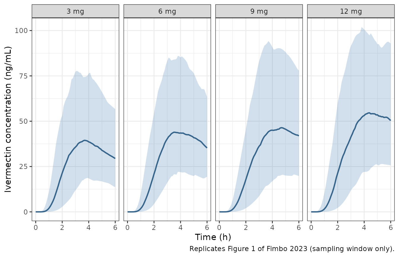
Replicates the structure of Figure 1 of Fimbo 2023: simulated 5th, 50th and 95th percentiles of ivermectin concentration by dose pool over the 0-6 h sampling window used in the study.
# The observed AUC0-6 and Cmax in Table 3 sit inside the simulated cohort's
# central range. Compare the cohort MEDIAN, which is robust to the tails and,
# for a log-normal eta, is the quantity the typical-value prediction estimates.
obs_tab3 <- tibble::tribble(
  ~pool,   ~cmax_obs,
  "3 mg",         40,
  "6 mg",         52,
  "9 mg",         51,
  "12 mg",        57
)

cmax_sim <- sim |>
  dplyr::filter(time <= 6) |>
  dplyr::group_by(pool, id) |>
  dplyr::summarise(cmax = max(Cc), .groups = "drop") |>
  dplyr::group_by(pool) |>
  dplyr::summarise(cmax_med = median(cmax), .groups = "drop") |>
  dplyr::left_join(obs_tab3, by = "pool") |>
  dplyr::mutate(pct = 100 * (cmax_med - cmax_obs) / cmax_obs)

cmax_sim |>
  dplyr::transmute("Dose pool" = pool,
                   "Simulated median Cmax (ng/mL)" = round(cmax_med, 1),
                   "Observed Cmax, Table 3 (ng/mL)" = cmax_obs,
                   "Difference (%)" = round(pct, 1)) |>
knitr::kable(caption = "Cohort median Cmax over 0-6 h vs the observed column of Fimbo 2023 Table 3.")| Dose pool | Simulated median Cmax (ng/mL) | Observed Cmax, Table 3 (ng/mL) | Difference (%) |
|---|---|---|---|
| 3 mg | 41.4 | 40 | 3.4 |
| 6 mg | 47.2 | 52 | -9.2 |
| 9 mg | 48.8 | 51 | -4.4 |
| 12 mg | 57.5 | 57 | 0.9 |
# Robust, cohort-derived: assert on the centre and an envelope, never on an
# extreme. A mis-transcribed volume or dose moves the whole distribution.
stopifnot(
  abs(median(cmax_sim$pct)) < 20,
  max(abs(cmax_sim$pct))    < 30
)
# The MTT mixture shifts absorption timing but must NOT change total exposure,
# because MTT only reshapes the input function -- it does not scale its area.
# This is a structural property of the transit chain and holds per cohort.
by_mix <- sim |>
  dplyr::filter(pool == "12 mg") |>
  dplyr::group_by(MIX_LONG_MTT, id) |>
  dplyr::summarise(auc72 = trapz(time, Cc), tmax = time[which.max(Cc)],
                   .groups = "drop") |>
  dplyr::group_by(MIX_LONG_MTT) |>
  dplyr::summarise(auc72 = median(auc72), tmax = median(tmax), .groups = "drop")

knitr::kable(by_mix, digits = 1,
caption = "Long-MTT subpopulation (1) vs reference (0), 12 mg pool: later peak, same area.")| MIX_LONG_MTT | auc72 | tmax |
|---|---|---|
| 0 | 1291.9 | 4.4 |
| 1 | 1278.5 | 5.9 |
auc_ratio <- by_mix$auc72[by_mix$MIX_LONG_MTT == 1] /
  by_mix$auc72[by_mix$MIX_LONG_MTT == 0]
stopifnot(
  # Areas agree; the 10% band admits cohort sampling noise between the two
  # subgroups (the long-MTT group is only ~16% of the cohort).
  abs(auc_ratio - 1) < 0.10,
  # The long-MTT group peaks later. MTT nearly doubles (x1.9695), so this is a
  # large, reliably-signed effect, not a near-zero one.
  by_mix$tmax[by_mix$MIX_LONG_MTT == 1] > by_mix$tmax[by_mix$MIX_LONG_MTT == 0]
)
Height-based versus weight-based dosing
Fimbo 2023’s second conclusion is that height-pole dosing underdoses heavier adults: the top pole caps the dose at 12 mg for everyone taller than 159 cm, so mg/kg falls as weight rises, whereas the WHO 200 ug/kg target rounded to whole 3 mg tablets tracks weight. The paper reports that 23%, 30%, and 100% of people weighing 61-70, 71-80, and over 80 kg were underdosed (below 150 ug/kg) under height-based dosing, versus 0% in every one of those bands under weight-based dosing (Table S1).
The comparison below is restricted to the weight bands from 51 kg upward. That restriction matters: the 12 mg dose is the top height pole, given to everyone taller than 159 cm, so it is only the applicable height-based dose for adults. A 35 kg person is short enough to fall on the 6 or 9 mg pole, and assigning them 12 mg would be counterfactual – it would manufacture a large apparent over-exposure at low weight that the height-pole system never produces. Because the model carries weight and not height, and no height-weight relationship is published for this cohort, the honest comparison is over the weight range where the top pole genuinely applies. This is also exactly the range the paper’s claim is about (above versus below 70 kg).
bands <- tibble::tribble(
  ~band,      ~wt,
  "51-60 kg",  55,
  "61-70 kg",  65,
  "71-80 kg",  75,
  ">80 kg",    85
)

# Weight-based: 200 ug/kg rounded to the nearest whole 3 mg tablet, exactly as
# Fimbo 2023 describes in "Evaluation of ivermectin height-based dosing".
bands <- bands |>
  dplyr::mutate(
    dose_height = 12,                                   # top height pole cap
    dose_weight = pmax(3, round(0.2 * wt / 3) * 3),     # 200 ug/kg -> whole tablets
    ugkg_height = 1000 * dose_height / wt,
    ugkg_weight = 1000 * dose_weight / wt
  )

ev_band <- dplyr::bind_rows(lapply(seq_len(nrow(bands)), function(i) {
  b <- bands[i, ]
  dplyr::bind_rows(lapply(c("Height-based", "Weight-based"), function(strat) {
    amt <- if (strat == "Height-based") b$dose_height else b$dose_weight
    idx <- i + ifelse(strat == "Height-based", 0L, 100L)
    dplyr::bind_rows(
      tibble::tibble(id = idx, time = 0, amt = amt, evid = 1L, cmt = "depot"),
      tibble::tibble(id = idx, time = grid_t, amt = NA_real_, evid = 0L,
                     cmt = "central")
    ) |>
      dplyr::mutate(band = b$band, strategy = strat, WT = b$wt,
                    DOSE_3MG = 0L, MIX_LONG_MTT = 0L)
  }))
})) |>
  dplyr::arrange(id, time, dplyr::desc(evid))

stopifnot(!anyDuplicated(unique(ev_band[, c("id", "time", "evid")])))

sim_band <- rxode2::rxSolve(rxode2::zeroRe(mod), events = ev_band,
                            keep = c("band", "strategy", "WT")) |>
  as.data.frame()
#> ℹ omega/sigma items treated as zero: 'etalcl', 'etalvc', 'etalq', 'etalvp', 'etalmtt', 'etalfdepot'
#> Warning: multi-subject simulation without without 'omega'

auc_band <- sim_band |>
  dplyr::group_by(band, strategy, WT) |>
  dplyr::summarise(auc = trapz(time, Cc), .groups = "drop") |>
  dplyr::mutate(band = factor(band, levels = bands$band))
ggplot(auc_band, aes(band, auc, colour = strategy, group = strategy)) +
  geom_line(linewidth = 0.9) +
  geom_point(size = 2.4) +
  labs(x = NULL, y = "AUC(0-72 h) (h*ng/mL)", colour = NULL,
       caption = "Replicates Figure 2 of Fimbo 2023.") +
  theme_bw() +
  theme(axis.text.x = element_text(angle = 30, hjust = 1),
        legend.position = "top")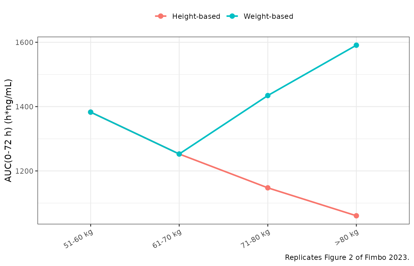
Replicates the message of Figure 2 of Fimbo 2023: typical-value AUC(0-72 h) by weight band under the 12 mg height-pole cap versus 200 ug/kg rounded to whole 3 mg tablets.
h <- auc_band |> dplyr::filter(strategy == "Height-based") |>
  dplyr::arrange(WT)
w <- auc_band |> dplyr::filter(strategy == "Weight-based") |>
  dplyr::arrange(WT)

# Deterministic (zeroRe, fixed band weights), so these are exact bounds.
#
# The gate encodes the paper's actual claim, which is DIRECTIONAL, not a
# flatness claim: "contrary to weight-based dosing, height-based dosing results
# in relatively lower AUC0-inf for individuals weighing greater than 70 kg
# compared to those weighing less than 70 kg" (Fimbo 2023 Results, Figure 2).
#
# Note it would be wrong to assert that weight-based dosing gives a FLATTER
# exposure profile than height-based dosing. It does not, and the model says so:
# rounding 200 ug/kg to whole 3 mg tablets makes the realised mg/kg jump around
# (171-218 ug/kg across these bands), so the weight-based spread is comparable
# to the height-based one. What weight-based dosing does is keep everyone above
# the 150 ug/kg efficacy threshold; it does not equalise exposure.
mean_gt70 <- function(d) mean(d$auc[d$WT > 70])
mean_le70 <- function(d) mean(d$auc[d$WT <= 70])

stopifnot(
  # Under the fixed 12 mg cap, AUC must fall monotonically with weight, because
  # CL/F rises allometrically while the dose does not rise at all. This is exact
  # and structural -- it goes red on a wrong allometric exponent or reference.
  all(diff(h$auc) < 0),
  # The paper's claim, height-based arm: heavier individuals get LESS exposure.
  mean_gt70(h) < mean_le70(h),
  # The paper's claim, weight-based arm: the pattern is reversed ("contrary to
  # weight-based dosing"), so heavier individuals do NOT lose exposure.
  mean_gt70(w) > mean_le70(w),
  # The paper's arithmetic claim: everyone above 80 kg is underdosed
  # (< 150 ug/kg) by the 12 mg cap, and nobody is under weight-based dosing.
  bands$ugkg_height[bands$band == ">80 kg"] < 150,
  all(bands$ugkg_weight >= 150)
)

bands |>
  dplyr::transmute("Weight band" = band,
                   "Height-based dose (mg)" = dose_height,
                   "Height-based (ug/kg)" = round(ugkg_height),
                   "Weight-based dose (mg)" = dose_weight,
                   "Weight-based (ug/kg)" = round(ugkg_weight)) |>
knitr::kable(caption = "Dose per kg by weight band under the two strategies. 150 ug/kg is the efficacy threshold Fimbo 2023 uses.")| Weight band | Height-based dose (mg) | Height-based (ug/kg) | Weight-based dose (mg) | Weight-based (ug/kg) |
|---|---|---|---|---|
| 51-60 kg | 12 | 218 | 12 | 218 |
| 61-70 kg | 12 | 185 | 12 | 185 |
| 71-80 kg | 12 | 160 | 15 | 200 |
| >80 kg | 12 | 141 | 18 | 212 |
Assumptions and deviations
Cohort size. The virtual cohort uses 200 subjects per dose pool rather than the published 12 / 49 / 159 / 248, to keep Monte-Carlo noise out of the cohort-level assertions while respecting the 200-per-arm cap. The typical-value comparisons against Table 3 do not depend on cohort size at all.
Weight distributions are drawn as
Normal(mean, SD)per dose pool from Fimbo 2023 Table 1 and truncated to [15, 95] kg. The paper reports only mean and SD, not the distributional shape; the lower truncation reflects the programme’s stated 15 kg eligibility floor. Truncation shifts the 3 mg pool’s realised mean slightly upward (its mean of 19.92 kg is only 1.5 SD above the floor); the 9 and 12 mg pools are essentially unaffected.The comparison target is a typical-value prediction, the published column is a mean over individual estimates. Fimbo 2023 Table 3’s “model estimated” values are summaries of per-subject empirical-Bayes estimates from the original dataset. With only three post-dose samples per subject the etas are substantially shrunk, so that mean sits close to a typical-value prediction but is not identical to one. This is the main reason the AUC comparison agrees to within roughly 5% rather than exactly, and it is why the cohort-level checks compare medians rather than means: for a log-normal eta the cohort mean of
1/CLis inflated byexp(omega^2 / 2)while the median is not.Height is not modelled, so the dosing comparison is restricted to adults. The paper assigns dose by height pole, but the model carries weight, not height, and no height-weight relationship is published for this cohort. The height-versus-weight section therefore compares the 12 mg top-pole cap against weight-based dosing at fixed band weights, rather than reconstructing individual pole assignments. It covers only the 51 kg and heavier bands, because the 12 mg pole applies to people taller than 159 cm: assigning 12 mg to a 35 kg child would be counterfactual and would fabricate an over-exposure at low weight that the pole system does not produce.
Weight-based dosing is not “flatter”, and the vignette does not claim it is. An earlier draft of this vignette asserted that weight-based dosing keeps AUC flatter across weight bands than height-based dosing. The model falsifies that: rounding the WHO 200 ug/kg target to whole 3 mg tablets makes the realised dose intensity swing between 171 and 218 ug/kg, so the weight-based AUC spread is comparable to the height-based one. What weight-based dosing achieves – and all the paper claims for it – is that nobody falls below the 150 ug/kg efficacy threshold, and that exposure stops declining with weight. The gate now tests that directional claim rather than a flatness claim.
Mixture assignment.
MIX_LONG_MTTis a latent class, not an observable patient characteristic. The cohort draws it asBernoulli(0.1606); the typical-value simulations set it to 0 (the 83.9% majority class).IIV correlations are unreported. Data S3 declares
$OMEGA BLOCK(4)over CL, Vc, Q and Vp with all six off-diagonal initial estimates set to 0. A NONMEMBLOCKwithoutFIXestimates its covariances, so the deposited stream implies six correlation parameters were estimated – but neither Table 2 nor Table S3 reports a single covariance or correlation, and Table S3’s variability columns are diagonals only (ECL,EVC,EQ,EVP,EMTT,EF1). The estimated covariances are therefore a genuine reporting gap. The model file encodes the four IIVs as independent (diagonal) because that is the only structure the published numbers support; a user reproducing individual-level correlation structure should treat this as a known limitation rather than as a claim that the covariances were zero.MTT mixture effect: 97.4% in prose, 96.95% in the table. Fimbo 2023’s Results text describes “a subpopulation (16% of the studied population) with 97.4% higher MTT”, but Table 2 and Table S3
run15both give the estimate as 0.9695, i.e. 96.95%. The abstract rounds it to “97%”. The model file encodes the table value (0.9695), since the parameter table is the authoritative source for a fitted estimate and the prose figure appears nowhere else.Age range discrepancy. Fimbo 2023 Methods states participants were “aged between 5- and 78 years old”, but the per-weight-band age ranges in Table S1 extend to 90 and 91 years. The model’s
populationmetadata records the Methods range and flags the discrepancy. Age is not a covariate in the final model, so nothing downstream depends on which reading is correct.Albendazole. Every participant also received albendazole 400 mg, and the paper notes albendazole may compete for CYP3A4/5. No albendazole term is in the model, so the ivermectin parameters here are conditional on co-administration with albendazole.
No non-paper-derived parameter values. Every value in the model file comes from Fimbo 2023 Table 2, Table S3, or the Data S3 NONMEM control stream. The structural model was adapted from Duthaler 2019 via the NONMEM PRIOR subroutine, but all encoded estimates are Fimbo 2023’s own; Duthaler’s prior values (
$THETA (7.67 FIXED) (89.13 FIXED) (19.0 FIXED) (234 FIXED)) are deliberately not used.