Bamlanivimab + etesevimab PK and SARS-CoV-2 viral dynamics (Chigutsa 2021)

Model and source

• Citation: Chigutsa E, O’Brien L, Ferguson-Sells L, Long A, Chien J. Population Pharmacokinetics and Pharmacodynamics of the Neutralizing Antibodies Bamlanivimab and Etesevimab in Patients With Mild to Moderate COVID-19 Infection. Clin Pharmacol Ther. 2021;110(5):1302-1310. doi:10.1002/cpt.2420. PK parameters are Supplementary Table S2, viral-dynamic parameters are Table 1, and the viral-dynamic NONMEM control stream is Supplementary Material S1.
• Article (open access): https://doi.org/10.1002/cpt.2420
• Supporting Information: Table S1 (demographics), Table S2 (PK parameters) and the NONMEM control stream of the viral-dynamic model.

Bamlanivimab and etesevimab are neutralizing IgG1 antibodies against the receptor-binding domain of the SARS-CoV-2 spike protein. Chigutsa 2021 analysed them sequentially. First, each antibody got its own two-compartment PK model. Then the individual post hoc PK predictions drove a target-cell-limited viral-dynamic model of nasopharyngeal viral load. In that model both antibodies raise the virus elimination rate.

The package ships all three parts as one model, Chigutsa_2021_bamlanivimab_etesevimab. This matches the published viral-dynamic control stream, whose $DES block carries both PK systems next to the viral states. The two PK systems share no parameters, so the model can also be used for either antibody’s PK alone.

mod <- rxode2::rxode2(readModelDb("Chigutsa_2021_bamlanivimab_etesevimab"))
#> ℹ parameter labels from comments will be replaced by 'label()'
mod_typ <- rxode2::zeroRe(mod)

Population

The PK analysis pooled BLAZE-1 (NCT04427501) and BLAZE-4 (NCT04634409), two phase II dose-ranging, placebo-controlled trials in outpatients with mild to moderate COVID-19. It also included 18 hospitalized patients with severe COVID-19 (J2W-MC-PYAA) and 20 healthy participants (J2Z-MC-PGAA). The data were 5915 bamlanivimab concentrations from 1899 participants and 4961 etesevimab concentrations from 1498 participants. The viral-dynamic analysis used 17,805 viral-load measurements from 2970 BLAZE-1/-4 participants, 1047 of whom received placebo. Single IV doses ranged from 175 to 7000 mg bamlanivimab, alone or with 350 to 2800 mg etesevimab.

In the viral-load population (Table S1), median body weight was 87.8 kg (range 41.4-220) and median age 50 years (12-94). 52.4% were female and 85.9% White, 7.2% Black and 3.9% Asian. 20.2% had mild hepatic impairment. Median baseline viral load was 5.30 log10 units, where one unit is (40 - Ct)/log2(10).

Source trace

Quantity	Value	Source
Bamlanivimab CL, Q, V1, V2 (70 kg)	0.231 L/d, 0.281 L/d, 2.68 L, 2.68 L	Table S2
Etesevimab CL, Q, V1, V2 (70 kg)	0.111 L/d, 0.308 L/d, 2.45 L, 2.18 L	Table S2
Weight exponent on CL and Q / on V1 and V2	0.81 fixed / 1 fixed	Table S2 footnotes a, b
IIV CL, V1 (bamlanivimab; etesevimab)	25.1%, 28.9%; 28.4%, 30.7%	Table S2
Proportional residual error (bam; ete)	19.0%; 18.3%	Table S2
Target-cell pool	4 x 10^8 fixed (stream: 400 in units of 1e6)	Table 1; stream THETA(1)
Log10 viral load at symptom onset	7.60	Table 1
beta, PV, CV, DI	5.23e-7, 0.0844 /d, 1.42 /d, 0.290 /d	Table 1
Emax, EC50 (bamlanivimab)	0.462, 0.467 ug/mL	Table 1
Etesevimab EC50 = 3 x bamlanivimab EC50	fixed	Results “Viral dynamic modeling”; stream $DES
IIV beta, PV, CV and their correlations	2526%, 47.2%, 85.4%; 0.939, 0.344, 0.359	Table 1
IIV viral load at onset, DI, Emax, EC50	15% fixed each	Table 1; stream $OMEGA 0.0225 FIX
Additive residual error (log10 viral load)	0.939	Table 1; stream $ERROR
Two-compartment PK ODEs	–	Methods; stream $DES A(1), A(2), A(6), A(7)
Target-cell-limited viral ODEs	–	Methods equations; stream $DES A(3)-A(5)
CV(t) = CV + Emax C1/(EC50 + C1) + Emax C2/(3 EC50 + C2)	–	Table 1 footnote c; stream TEFF, CBTEFF
log10 viral load = log10(virus x 1e6), floored at 1e-5	–	stream $ERROR

Typical-value viral dynamics

Replicating Table 2

Table 2 of the paper gives the model-predicted reduction in viral load relative to placebo after 700 mg bamlanivimab plus 1400 mg etesevimab given 1, 4 or 10 days after symptom onset. The model clock starts at symptom onset. The time-weighted-average windows “days 0 to 7” and “days 0 to 11” start on the day of treatment. (A window starting at symptom onset does not reproduce the table.) The infusion duration is not reported, so a 1-hour infusion is used here.

# One subject with observations on a fine grid; dvid = 3 nominates the
# log10_viral_load endpoint, and every endpoint comes back as a column.
make_events <- function(t_dose = NA, bam = 0, ete = 0, wt = 70, id = 1,
                        times = seq(0, 30, by = 0.01)) {
  obs <- data.frame(
    id = id, time = times, amt = 0, rate = 0, evid = 0L,
    cmt = "virus", dvid = 3L, WT = wt
  )
  if (is.na(t_dose)) {
    return(obs)
  }
  dose <- data.frame(
    id = id, time = t_dose, amt = c(bam, ete), rate = c(bam, ete) * 24,
    evid = 1L, cmt = c("central", "central_ete"), dvid = NA_integer_, WT = wt
  )
  dose <- dose[dose$amt > 0, ]
  ev <- rbind(dose, obs)
  ev[order(ev$id, ev$time, -ev$evid), ]
}

solve_typ <- function(ev) {
  as.data.frame(rxode2::rxSolve(mod_typ, ev, returnType = "data.frame"))
}

# Trapezoidal time-weighted average of y over [lo, hi]
twa <- function(t, y, lo, hi) {
  keep <- t >= lo - 1e-9 & t <= hi + 1e-9
  tt <- t[keep]
  yy <- y[keep]
  sum(diff(tt) * (head(yy, -1) + tail(yy, -1)) / 2) / (hi - lo)
}

placebo <- solve_typ(make_events())
#> ℹ omega/sigma items treated as zero: 'etalcl', 'etalvc', 'etalcl_ete', 'etalvc_ete', 'etalvirus0', 'etalbeta', 'etalp', 'etalc', 'etaldelta', 'etalemax', 'etalec50'

table2 <- lapply(c(1, 4, 10), function(td) {
  trt <- solve_typ(make_events(t_dose = td, bam = 700, ete = 1400))
  data.frame(
    day = td,
    twa7 = twa(placebo$time, placebo$log10_viral_load, td, td + 7) -
      twa(trt$time, trt$log10_viral_load, td, td + 7),
    twa11 = twa(placebo$time, placebo$log10_viral_load, td, td + 11) -
      twa(trt$time, trt$log10_viral_load, td, td + 11),
    maxred = max(placebo$log10_viral_load - trt$log10_viral_load)
  )
}) |>
  bind_rows()
#> ℹ omega/sigma items treated as zero: 'etalcl', 'etalvc', 'etalcl_ete', 'etalvc_ete', 'etalvirus0', 'etalbeta', 'etalp', 'etalc', 'etaldelta', 'etalemax', 'etalec50'
#> ℹ omega/sigma items treated as zero: 'etalcl', 'etalvc', 'etalcl_ete', 'etalvc_ete', 'etalvirus0', 'etalbeta', 'etalp', 'etalc', 'etaldelta', 'etalemax', 'etalec50'
#> ℹ omega/sigma items treated as zero: 'etalcl', 'etalvc', 'etalcl_ete', 'etalvc_ete', 'etalvirus0', 'etalbeta', 'etalp', 'etalc', 'etaldelta', 'etalemax', 'etalec50'

published <- data.frame(
  day = c(1, 4, 10),
  twa7_pub = c(1.15, 0.70, 0.25),
  twa11_pub = c(0.99, 0.55, 0.24),
  maxred_pub = c(1.82, 1.15, 0.28)
)

t2 <- left_join(table2, published, by = "day")
t2 |>
  mutate(across(where(is.double), \(x) round(x, 2))) |>
  select(day, twa7_pub, twa7, twa11_pub, twa11, maxred_pub, maxred) |>
  rename(
    "Treatment day (from symptom onset)" = day,
    "TWA days 0-7, paper" = twa7_pub,
    "TWA days 0-7, model" = twa7,
    "TWA days 0-11, paper" = twa11_pub,
    "TWA days 0-11, model" = twa11,
    "Max reduction, paper" = maxred_pub,
    "Max reduction, model" = maxred
  ) |>
  knitr::kable(caption = "Replicates Table 2 of Chigutsa 2021: log10 reduction relative to placebo.")

Replicates Table 2 of Chigutsa 2021: log10 reduction relative to placebo.

Treatment day (from symptom onset)	TWA days 0-7, paper	TWA days 0-7, model	TWA days 0-11, paper	TWA days 0-11, model	Max reduction, paper	Max reduction, model
1	1.15	1.17	0.99	0.99	1.82	1.82
4	0.70	0.71	0.55	0.55	1.15	1.15
10	0.25	0.25	0.24	0.24	0.28	0.28

All nine cells are deterministic typical-value solves, so the comparison is tight. The paper prints two decimals. The largest gap (0.017 log10, TWA days 0-7 after treatment on day 1) is within rounding plus the unreported infusion duration.

stopifnot(
  all(abs(t2$twa7 - t2$twa7_pub) < 0.03),
  all(abs(t2$twa11 - t2$twa11_pub) < 0.03),
  all(abs(t2$maxred - t2$maxred_pub) < 0.03)
)

The in vivo IC90 values in the Abstract follow directly from the EC50s with Hill = 1 (IC90 = 9 x EC50). The same holds for the 25.2 ug/mL used in the Figure S2 sensitivity analysis, where etesevimab is assumed 6-fold less potent than bamlanivimab.

ec50 <- exp(mod$theta[["lec50"]])
ratio <- mod$theta[["ec50_ratio_ete"]]
ic90 <- c(bamlanivimab = 9 * ec50, etesevimab = 9 * ec50 * ratio, etesevimab_6x = 9 * ec50 * 6)
round(ic90, 1)
#>  bamlanivimab    etesevimab etesevimab_6x 
#>           4.2          12.6          25.2
stopifnot(
  abs(ic90[["bamlanivimab"]] - 4.2) < 0.05,
  abs(ic90[["etesevimab"]] - 12.6) < 0.05,
  abs(ic90[["etesevimab_6x"]] - 25.2) < 0.05
)

Replicating Figure 4: timing and monotherapy vs combination

fig4 <- bind_rows(
  lapply(c(1, 4, 10), function(td) {
    bind_rows(
      solve_typ(make_events(t_dose = td, bam = 700)) |>
        mutate(arm = "Bamlanivimab 700 mg"),
      solve_typ(make_events(t_dose = td, bam = 700, ete = 1400)) |>
        mutate(arm = "Bamlanivimab 700 mg + etesevimab 1400 mg")
    ) |>
      mutate(t_dose = paste("Treated on day", td))
  })
) |>
  left_join(
    placebo |> select(time, placebo = log10_viral_load),
    by = "time"
  ) |>
  mutate(difference = log10_viral_load - placebo)
#> ℹ omega/sigma items treated as zero: 'etalcl', 'etalvc', 'etalcl_ete', 'etalvc_ete', 'etalvirus0', 'etalbeta', 'etalp', 'etalc', 'etaldelta', 'etalemax', 'etalec50'
#> ℹ omega/sigma items treated as zero: 'etalcl', 'etalvc', 'etalcl_ete', 'etalvc_ete', 'etalvirus0', 'etalbeta', 'etalp', 'etalc', 'etaldelta', 'etalemax', 'etalec50'
#> ℹ omega/sigma items treated as zero: 'etalcl', 'etalvc', 'etalcl_ete', 'etalvc_ete', 'etalvirus0', 'etalbeta', 'etalp', 'etalc', 'etaldelta', 'etalemax', 'etalec50'
#> ℹ omega/sigma items treated as zero: 'etalcl', 'etalvc', 'etalcl_ete', 'etalvc_ete', 'etalvirus0', 'etalbeta', 'etalp', 'etalc', 'etaldelta', 'etalemax', 'etalec50'
#> ℹ omega/sigma items treated as zero: 'etalcl', 'etalvc', 'etalcl_ete', 'etalvc_ete', 'etalvirus0', 'etalbeta', 'etalp', 'etalc', 'etaldelta', 'etalemax', 'etalec50'
#> ℹ omega/sigma items treated as zero: 'etalcl', 'etalvc', 'etalcl_ete', 'etalvc_ete', 'etalvirus0', 'etalbeta', 'etalp', 'etalc', 'etaldelta', 'etalemax', 'etalec50'

placebo_panel <- tidyr::crossing(
  placebo |> select(time, log10_viral_load),
  t_dose = unique(fig4$t_dose)
) |>
  mutate(arm = "Placebo")

ggplot(bind_rows(fig4, placebo_panel), aes(time, log10_viral_load, colour = arm)) +
  geom_line() +
  facet_wrap(~t_dose) +
  coord_cartesian(xlim = c(0, 20)) +
  labs(
    x = "Days since onset of symptoms", y = "log10 viral load", colour = NULL,
    caption = "Replicates Figure 4 (top) of Chigutsa 2021."
  ) +
  theme_bw() +
  theme(legend.position = "bottom")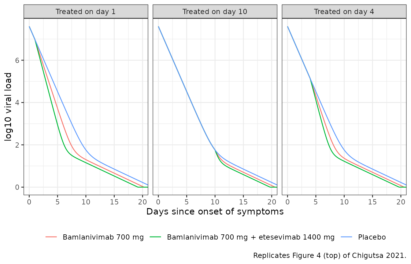

ggplot(fig4, aes(time, difference, colour = arm)) +
  geom_line() +
  facet_wrap(~t_dose) +
  coord_cartesian(xlim = c(0, 20)) +
  labs(
    x = "Days since onset of symptoms", y = "Difference from placebo (log10)",
    colour = NULL, caption = "Replicates Figure 4 (bottom) of Chigutsa 2021."
  ) +
  theme_bw() +
  theme(legend.position = "bottom")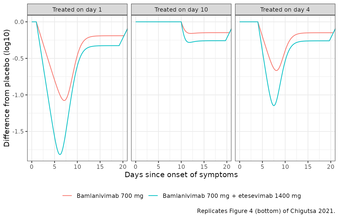

Adding etesevimab gives a further reduction beyond bamlanivimab alone. This matches the paper’s reading that bamlanivimab exposure already sits near its own Emax. The etesevimab term adds a second Emax.

day7 <- fig4 |>
  filter(abs(time - 7) < 1e-6, t_dose == "Treated on day 4") |>
  select(arm, log10_viral_load)
day7
#>                                        arm log10_viral_load
#> 1                      Bamlanivimab 700 mg         2.726656
#> 2 Bamlanivimab 700 mg + etesevimab 1400 mg         2.205945
stopifnot(
  day7$log10_viral_load[day7$arm == "Bamlanivimab 700 mg + etesevimab 1400 mg"] <
    day7$log10_viral_load[day7$arm == "Bamlanivimab 700 mg"] - 0.3
)

Replicating Figure 3: body weight

Figure 3 compares a 40 kg and a 220 kg patient given 700/1400 mg. Here the dose is on day 4 after symptom onset (the trials’ median). Serum concentrations differ several-fold, but both stay far above the IC90 for weeks. The viral-load curves overlap.

fig3 <- bind_rows(
  solve_typ(make_events(t_dose = 4, bam = 700, ete = 1400, wt = 40, times = seq(0, 40, by = 0.05))) |>
    mutate(weight = "40 kg"),
  solve_typ(make_events(t_dose = 4, bam = 700, ete = 1400, wt = 220, times = seq(0, 40, by = 0.05))) |>
    mutate(weight = "220 kg")
)
#> ℹ omega/sigma items treated as zero: 'etalcl', 'etalvc', 'etalcl_ete', 'etalvc_ete', 'etalvirus0', 'etalbeta', 'etalp', 'etalc', 'etaldelta', 'etalemax', 'etalec50'
#> ℹ omega/sigma items treated as zero: 'etalcl', 'etalvc', 'etalcl_ete', 'etalvc_ete', 'etalvirus0', 'etalbeta', 'etalp', 'etalc', 'etaldelta', 'etalemax', 'etalec50'

fig3 |>
  select(time, weight, `log10 viral load` = log10_viral_load, `Bamlanivimab (ug/mL)` = Cc, `Etesevimab (ug/mL)` = Cc_ete) |>
  pivot_longer(-c(time, weight)) |>
  ggplot(aes(time, value, colour = weight, linetype = weight)) +
  geom_line() +
  facet_wrap(~name, ncol = 1, scales = "free_y") +
  labs(x = "Days since onset of symptoms", y = NULL, colour = "Body weight", linetype = "Body weight",
       caption = "Replicates Figure 3 of Chigutsa 2021 (dose on day 4).") +
  theme_bw()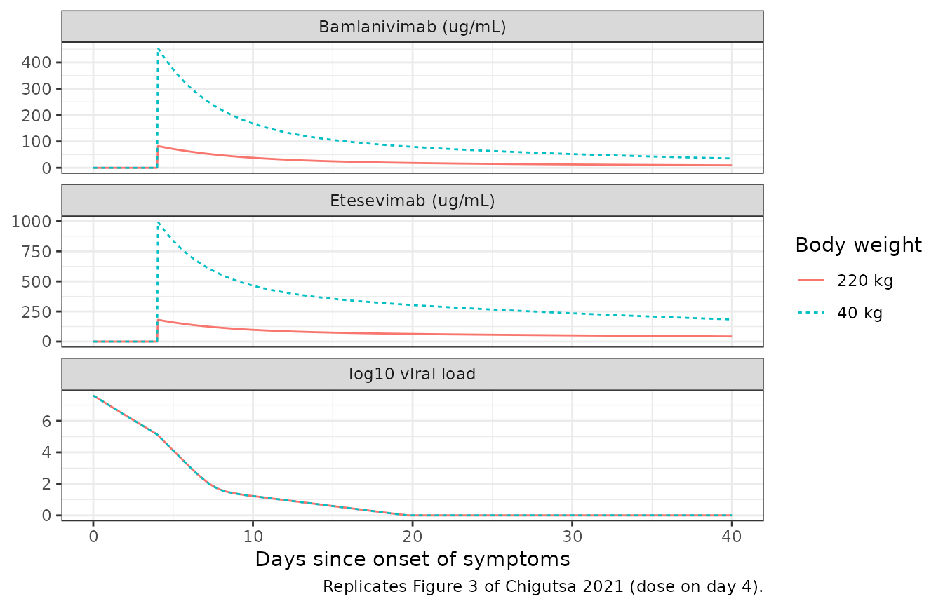

vl_gap <- fig3 |>
  select(time, weight, log10_viral_load) |>
  pivot_wider(names_from = weight, values_from = log10_viral_load)
max_gap <- max(abs(vl_gap$`40 kg` - vl_gap$`220 kg`))
c28 <- fig3 |> filter(abs(time - 32) < 1e-6, weight == "220 kg")
c(max_vl_gap = max_gap, bam_day28_220kg = c28$Cc, ete_day28_220kg = c28$Cc_ete)
#>      max_vl_gap bam_day28_220kg ete_day28_220kg 
#>     0.006522482    11.985008412    49.350054086
stopifnot(
  max_gap < 0.05,
  c28$Cc > ic90[["bamlanivimab"]],
  c28$Cc_ete > ic90[["etesevimab"]]
)

Stochastic PK: virtual cohort

Virtual cohort

The cohort is 200 virtual patients. Body weight is drawn log-normally around the viral-load population’s median of 87.8 kg, and draws outside the observed 41.4-220 kg range are rejected and redrawn. Each patient gets 700 mg bamlanivimab plus 1400 mg etesevimab on day 4 after symptom onset. Serum is sampled on the trials’ schedule, extended to a dense grid for NCA.

rxode2::rxSetSeed(20211)
n_sub <- 200
draw_wt <- function(n) {
  out <- numeric(0)
  while (length(out) < n) {
    w <- exp(rnorm(n, log(87.8), 0.25))
    out <- c(out, w[w >= 41.4 & w <= 220])
  }
  out[seq_len(n)]
}
wts <- draw_wt(n_sub)
summary(wts)
#>    Min. 1st Qu.  Median    Mean 3rd Qu.    Max. 
#>   45.69   76.51   89.90   92.99  106.92  174.85

t_dose <- 4
obs_times <- t_dose + c(0, 1 / 24, 0.25, 0.5, 1, 2, 4, 7, 10, 14, 21, 28, 35, 42, 56, 70, 84)
cohort_ev <- lapply(seq_len(n_sub), function(i) {
  make_events(t_dose = t_dose, bam = 700, ete = 1400, wt = wts[i], id = i, times = c(0, obs_times))
}) |>
  bind_rows()

sim <- rxode2::rxSolve(mod, cohort_ev, returnType = "data.frame") |>
  as.data.frame() |>
  mutate(tad = time - t_dose, treatment = "700 mg bamlanivimab + 1400 mg etesevimab")

Replicating Figure 5 (right): PK profiles against the IC90

pk_long <- sim |>
  filter(tad >= 0) |>
  select(id, tad, Bamlanivimab = Cc, Etesevimab = Cc_ete) |>
  pivot_longer(c(Bamlanivimab, Etesevimab), names_to = "drug", values_to = "conc")

pk_sum <- pk_long |>
  group_by(drug, tad) |>
  summarise(
    median = median(conc), lo = quantile(conc, 0.05), hi = quantile(conc, 0.95),
    .groups = "drop"
  )
ic90_band <- data.frame(
  drug = c("Bamlanivimab", "Etesevimab"),
  lo = c(3.2, 9.7), hi = c(4.3, 12.8)
)

ggplot(pk_sum, aes(tad, median)) +
  geom_ribbon(aes(ymin = lo, ymax = hi), alpha = 0.3) +
  geom_line() +
  geom_rect(
    data = ic90_band, inherit.aes = FALSE,
    aes(xmin = -Inf, xmax = Inf, ymin = lo, ymax = hi), alpha = 0.3, fill = "red"
  ) +
  facet_wrap(~drug) +
  scale_y_log10() +
  labs(
    x = "Days after dose", y = "Serum concentration (ug/mL)",
    caption = "Replicates Figure 5 (right) of Chigutsa 2021: 90% PI; red band = 95% CI of the IC90."
  ) +
  theme_bw()
#> Warning in scale_y_log10(): log-10 transformation introduced infinite values.
#> log-10 transformation introduced infinite values.
#> log-10 transformation introduced infinite values.
#> log-10 transformation introduced infinite values.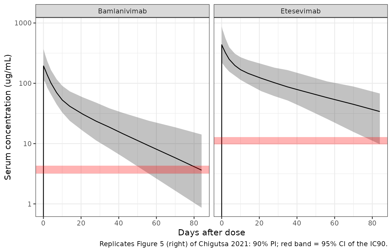

Figure 5 (left) reports that at least 90% of patients stay above the IC90 for 28 days after the authorized doses. The simulated day-28 proportions are shown below. The gate is on the day-28 median, which is far above the IC90; a threshold-crossing percentage is not a stable gate.

day28 <- pk_long |> filter(abs(tad - 28) < 1e-6)
day28 |>
  group_by(drug) |>
  summarise(
    median_conc = median(conc),
    pct_above_ic90 = 100 * mean(conc > ifelse(drug == "Bamlanivimab", ic90[["bamlanivimab"]], ic90[["etesevimab"]])),
    .groups = "drop"
  ) |>
  rename("Drug" = drug, "Median day-28 conc (ug/mL)" = median_conc, "% above IC90" = pct_above_ic90) |>
  knitr::kable(digits = 1)

Drug	Median day-28 conc (ug/mL)	% above IC90
Bamlanivimab	23.5	100
Etesevimab	102.4	100

stopifnot(
  median(day28$conc[day28$drug == "Bamlanivimab"]) > 3 * ic90[["bamlanivimab"]],
  median(day28$conc[day28$drug == "Etesevimab"]) > 3 * ic90[["etesevimab"]]
)

PKNCA validation

The paper reports one NCA-type quantity for each antibody: the terminal half-life, 20.9 days for bamlanivimab and 32.6 days for etesevimab (Results, “PK modeling”). The paper does not say which summary statistic this is. Here the simulated median is compared against it. The model predictions are used without residual error.

nca_one <- function(col, label) {
  conc <- sim |>
    filter(tad >= 0, !is.na(.data[[col]])) |>
    transmute(id, time = tad, conc = .data[[col]], treatment = label) |>
    distinct(id, time, .keep_all = TRUE)
  dose <- conc |>
    distinct(id, treatment) |>
    mutate(time = 0, amt = ifelse(label == "Bamlanivimab", 700, 1400))
  intervals <- data.frame(
    start = 0, end = Inf, cmax = TRUE, tmax = TRUE,
    auclast = TRUE, aucinf.obs = TRUE, half.life = TRUE
  )
  res <- PKNCA::pk.nca(PKNCA::PKNCAdata(
    PKNCA::PKNCAconc(conc, conc ~ time | treatment + id),
    PKNCA::PKNCAdose(dose, amt ~ time | treatment + id),
    intervals = intervals
  ))
  as.data.frame(res$result)
}

nca_res <- bind_rows(
  nca_one("Cc", "Bamlanivimab"),
  nca_one("Cc_ete", "Etesevimab")
)

reference <- data.frame(
  treatment = c("Bamlanivimab", "Etesevimab"),
  half.life = c(20.9, 32.6)
)

cmp <- ncaComparisonTable(
  nca_res, reference,
  by = "treatment", params = "half.life",
  units = c(half.life = "day")
)
knitr::kable(cmp)

NCA parameter	treatment	Reference	Simulated	% diff
t½ (day)	Bamlanivimab	20.9	20.8	-0.6%
t½ (day)	Etesevimab	32.6	33.7	+3.4%

hl <- nca_res |>
  filter(PPTESTCD == "half.life") |>
  group_by(treatment) |>
  summarise(median_hl = median(PPORRES), .groups = "drop") |>
  left_join(reference, by = "treatment") |>
  mutate(pct_diff = 100 * (median_hl - half.life) / half.life)
hl
#> # A tibble: 2 × 4
#>   treatment    median_hl half.life pct_diff
#>   <chr>            <dbl>     <dbl>    <dbl>
#> 1 Bamlanivimab      20.8      20.9   -0.643
#> 2 Etesevimab        33.7      32.6    3.39
stopifnot(all(abs(hl$pct_diff) < 10))

As a deterministic cross-check, the typical-value terminal half-life at each drug’s median body weight (85.7 kg bamlanivimab PK population, 87.8 kg etesevimab) is:

typ_hl <- function(cl, q, v1, v2, wt) {
  cl <- cl * (wt / 70)^0.81
  q <- q * (wt / 70)^0.81
  v1 <- v1 * wt / 70
  v2 <- v2 * wt / 70
  k10 <- cl / v1
  k12 <- q / v1
  k21 <- q / v2
  s <- k10 + k12 + k21
  log(2) / ((s - sqrt(s^2 - 4 * k10 * k21)) / 2)
}
th <- mod$theta
hl_typ <- c(
  bamlanivimab = typ_hl(exp(th[["lcl"]]), exp(th[["lq"]]), exp(th[["lvc"]]), exp(th[["lvp"]]), 85.7),
  etesevimab = typ_hl(exp(th[["lcl_ete"]]), exp(th[["lq_ete"]]), exp(th[["lvc_ete"]]), exp(th[["lvp_ete"]]), 87.8)
)
round(hl_typ, 1)
#> bamlanivimab   etesevimab 
#>         20.8         32.8
stopifnot(abs(hl_typ[["bamlanivimab"]] - 20.9) < 0.5, abs(hl_typ[["etesevimab"]] - 32.6) < 0.5)

Assumptions and deviations

• IIV scale. Tables 1 and S2 report IIV as %CV. The beta entry of 2526% is only consistent with CV = sqrt(exp(omega^2) - 1). The “15% Fixed” entries are OMEGA 0.0225 FIX in the control stream, which gives 15.1% on the same scale. So omega^2 = log(1 + CV^2) is used for every IIV term, including the PK terms of Table S2. The beta-PV-CV covariance block is rebuilt from the reported CVs and correlations.
• No PK correlations. Table S2 reports no CL-V1 correlation, so the PK etas are independent. IIV on Q and V2 was not estimated.
• Stream scale for the viral states. The control stream holds the virus and both cell pools in units of 1e6. The observation is log10(virus * 1e6), and the target-cell THETA is 400 FIX for the 4 x 10^8 cells in Table 1. The Table 1 values of beta, PV, CV and DI are the stream’s THETAs and are used on that scale. The Table 1 unit label for beta, ((copies/mL)^-1 day^-1), refers to the linear viral load before the 1e6 scaling. Table 2 is reproduced within rounding, which confirms this reading. Viral load at symptom onset (7.60 log10) enters the model as 10^(7.60 - 6).
• Target-cell IIV. The stream fixes the target-cell IIV to 0 ($OMEGA 0 FIX). The model therefore has no eta on the target-cell pool rather than a zero-variance eta.
• Emax is an additive rate. Table 1 labels Emax “fractional increase in CV”. Footnote c and the stream’s $DES both add Emax * C / (EC50 + C) to CV as a rate (per day). The equation is used here.
• Etesevimab potency. The etesevimab EC50 is fixed at three times the bamlanivimab EC50, as in the paper. It is exposed as ec50_ratio_ete = fixed(3) so the Figure S2 sensitivity analysis (6-fold) can be run by overriding it.
• Concentration floor. The stream floors the serum concentration at 1e-6 ug/mL when it is not positive. Its effect on the Emax terms is negligible, so it is omitted.
• Censoring. The analysis fitted viral loads below 0.05 log10 units with Beal’s M4 method, truncated at 0. This belongs to estimation, not to the structural model. To refit, supply the censoring columns in the data.
• Infusion duration. Not reported. Simulations here use a 1-hour infusion. It barely affects any of the comparisons above.
• Viral-load units. The dependent variable is (40 - Ct)/log2(10), a Ct-derived log10 scale relative to a cycle threshold of 40. It is not a calibrated copies/mL value.
• Weight distribution. Table S1 gives the weight median and range but no spread. The log-normal SD of 0.25 used for the virtual cohort is the maintainers’ assumption.