Selumetinib (Kollo 2026)
Source:vignettes/articles/Kollo_2026_selumetinib.Rmd
Kollo_2026_selumetinib.RmdModel and source
- Citation: Kollo Z, Kovacs J, Neely MN, Vasarhelyi B, Bruckner E, Szabo AJ, Garami M, Karvaly GB. A nonparametric population pharmacokinetic model of selumetinib in pediatric patients diagnosed with neurofibromatosis-I or plexiform neurofibromas. CPT Pharmacometrics Syst Pharmacol. 2026;15(1):e70156. doi:10.1002/psp4.70156
- Article: https://doi.org/10.1002/psp4.70156
- Supplement (Tables S1-S14): https://doi.org/10.1002/psp4.70156 Data S2
Kollo and colleagues built the first nonparametric
population PK model of selumetinib, in children treated for inoperable
neurofibromatosis type I (NF-1) or plexiform neurofibromas. The model
was fitted with the nonparametric adaptive grid (NPAG) algorithm in
Pmetrics. Eleven candidate models were compared; the winner (model C)
scaled the central volume linearly on total body weight,
V = V0 * WT.
The defining feature of this model is that between-subject
variability is not a parametric omega matrix. It is a
discrete joint distribution over 22 posterior support points (Table
S12), one per participant. That is why the packaged model file carries
no eta terms: writing a log-normal omega here would
contradict the paper’s central finding that parametric distributions
fail to capture selumetinib variability in this population. The support
points are reproduced below and drive every simulation in this
vignette.
Population
| Field | Value |
|---|---|
| species | human |
| n_subjects | 22 |
| n_studies | 1 |
| age_range | 61-192 months (5.1-16.0 years) |
| age_median | 140.5 months (11.7 years) |
| weight_range | 17.0-70.0 kg |
| weight_median | 39.35 kg |
| sex_female_pct | 45.5 |
| disease_state | inoperable neurofibromatosis type I (NF-1) or plexiform neurofibromas |
| dose_range | 10-35 mg orally per administration, q12h fixed or morning/evening alternating doses; initial doses set from body surface area per the Koselugo label and later individualised on clinical response and tolerability (Table S1) |
| regions | Hungary (single centre, Semmelweis University, Budapest) |
| notes | Twenty-eight children were recruited (July 2023-October 2024); 22 contributed 156 steady-state selumetinib concentrations (5-8 samples each) to model construction, and 6 further patients (S1-S5 and #18) contributed 10 samples to a limited external validation (Table S5). Patient #18 was excluded from model building because all of that patient’s concentrations fell in the absorption phase. Baseline demographics are in Table 1 and Table S1; laboratory values in Table S6. All participants had normal liver and renal function and took no chronic co-medication. The cohort covers 60 percent of the Hungarian paediatric NF-1 population receiving selumetinib. NOTE: weight_median is 39.35 kg computed from the individual weights in Table S1; the Results text states 33.4 kg, which cannot be correct because it lies below both sex-specific medians reported in Table 1 (males 44.3 kg, females 36.1 kg). See the vignette Errata. |
Twenty-eight children were recruited at the Pediatric Center, Semmelweis University (Budapest) between July 2023 and October 2024. Twenty-two contributed 156 steady-state selumetinib concentrations (5-8 samples each) to model construction; six further patients contributed 10 samples to a limited external validation (Table S5). Doses were individualised on clinical response: across the 28 recruited children, 14 took a fixed dose, 13 took alternating morning/evening doses, and one (patient S4) took alternating and then fixed doses at the first and second sampling occasion respectively (Methods 2.2; Table S1). Selumetinib was assayed in plasma by LC-MS/MS and reported in nmol/L.
Source trace
Every ini() entry carries an in-file comment naming its
source location in
inst/modeldb/specificDrugs/Kollo_2026_selumetinib.R. The
table collects them.
| Equation / parameter | Value | Source location |
|---|---|---|
lka (Ka) |
22.87 1/h | Table S14, Ka mean |
lkel (Ke) |
0.58 1/h | Table S14, Ke mean |
lvc (V0) |
0.50 L/kg | Table S14, V0 mean |
lk12 (KCP) |
1.32 1/h | Table S14, KCP mean |
lk21 (KPC) |
0.78 1/h | Table S14, KPC mean |
ltlag (Tlag1) |
0.62 h | Table S14, Tlag1 mean |
lfdepot (FA1) |
0.81 | Table S14, FA1 mean |
addSd |
2.1746 nmol/L | 2.474 (gamma, Results 3.1) x 0.879 (assay-error intercept, Results 3.1 / Figure 5E) |
propSd |
0.09203 | 2.474 (gamma, Results 3.1) x 0.0372 (assay-error slope, Results 3.1 / Figure 5E) |
vc <- exp(lvc) * WT |
n/a | Figure 4; Table S4 model C (V = V0 x WT) |
| Depot -> central, first order with lag and F | n/a | Figure 4 (F, Tlag, Ka) |
| Central <-> peripheral1 (KCP, KPC) | n/a | Figure 4 |
| Elimination from central (Ke) | n/a | Figure 4 |
| mg -> nmol dose conversion (MW 457.7 g/mol) | 2184.8 nmol/mg | Not in the paper; PubChem CID 10127622 (see Errata) |
The nonparametric support points (Table S12)
support <- tibble::tribble(
  ~point, ~Ka,      ~Ke,      ~V0,      ~KCP,     ~KPC,     ~Tlag1,   ~FA1,     ~prob,
  1L, 35.43558, 0.764815, 0.222757, 0.797045, 0.360794, 0.518729, 0.773015, 0.045502,
  2L,  1.915324, 0.880486, 0.201111, 0.535826, 0.095420, 0.408835, 0.565583, 0.045455,
  3L,  3.566975, 0.254133, 0.873045, 2.719549, 4.631848, 0.888647, 0.712266, 0.045455,
  4L, 19.19447, 0.473957, 0.399604, 0.456286, 0.064780, 0.580437, 0.918245, 0.090842,
  5L, 25.26479, 0.602355, 0.385131, 0.483356, 0.205264, 0.680340, 0.980238, 0.041136,
  6L, 19.85932, 0.686594, 0.388940, 0.332536, 0.201362, 0.582342, 0.990433, 0.045455,
  7L, 12.57163, 0.230077, 0.847987, 0.384977, 0.548601, 0.892162, 0.452210, 0.041435,
  8L, 74.99799, 0.624992, 0.408745, 0.303532, 0.125266, 0.870770, 0.950823, 0.045775,
  9L,  1.006084, 0.416966, 0.864161, 0.128864, 0.030534, 0.301141, 0.985592, 0.045455,
 10L,  4.762590, 0.602537, 0.252907, 0.375337, 0.036885, 0.541550, 0.651012, 0.045719,
 11L, 17.39898, 0.216717, 0.934062, 0.147145, 0.058857, 0.889672, 0.421624, 0.049474,
 12L, 50.51440, 0.540012, 0.366088, 0.440817, 0.314530, 0.282342, 0.999925, 0.045472,
 13L, 10.40697, 0.309562, 0.574038, 0.214586, 0.076487, 0.664666, 0.834925, 0.045455,
 14L, 47.47924, 0.432394, 0.398842, 0.278395, 0.189655, 0.681658, 0.846644, 0.045454,
 15L, 63.21599, 0.353357, 1.355650, 0.477032, 0.048721, 0.809913, 0.432428, 0.045455,
 16L,  1.395012, 1.939958, 0.191970, 1.995689, 0.134443, 0.416306, 0.999997, 0.045455,
 17L,  1.749552, 0.469133, 0.363803, 0.993825, 0.041366, 0.647234, 0.989847, 0.045455,
 18L, 30.24077, 0.501164, 0.157080, 1.206370, 0.266730, 0.546963, 0.999904, 0.045455,
 19L, 25.25033, 0.602355, 0.385131, 0.483356, 0.205264, 0.680340, 0.980238, 0.003735,
 20L,  7.586217, 0.189553, 0.907293, 8.549325, 7.827625, 0.977161, 0.617619, 0.045455,
 21L, 51.47915, 1.001312, 0.264024, 6.647797, 1.851095, 0.582755, 0.851397, 0.045455,
 22L,  3.101833, 0.832939, 0.249509, 1.157648, 0.062927, 0.360901, 0.960224, 0.045455
)
support$w <- support$prob / sum(support$prob)
stopifnot(nrow(support) == 22L, abs(sum(support$prob) - 1) < 1e-4)
Self-consistency check: Table S12 reproduces Table S14
Table S14 reports the mean, median, SD and CV% of each parameter’s
posterior. The Mean column must be the
probability-weighted mean of the support points.
Reproducing it verifies both the transcription above and the reading of
the two tables.
pars_np <- c("Ka", "Ke", "V0", "KCP", "KPC", "Tlag1", "FA1")
published_s14 <- c(Ka = 22.87, Ke = 0.58, V0 = 0.50, KCP = 1.32,
                   KPC = 0.78, Tlag1 = 0.62, FA1 = 0.81)

check_s14 <- tibble::tibble(
  Parameter          = pars_np,
  `Weighted mean of Table S12` = vapply(pars_np, function(p) sum(support$w * support[[p]]), numeric(1)),
  `Table S14 mean`   = unname(published_s14[pars_np])
) |>
  dplyr::mutate(`% diff` = 100 * (`Weighted mean of Table S12` - `Table S14 mean`) / `Table S14 mean`)

knitr::kable(check_s14, digits = c(0, 4, 2, 2),
caption = "Probability-weighted means of the 22 support points vs. the published summary.")| Parameter | Weighted mean of Table S12 | Table S14 mean | % diff |
|---|---|---|---|
| Ka | 22.8647 | 22.87 | -0.02 |
| Ke | 0.5816 | 0.58 | 0.28 |
| V0 | 0.5006 | 0.50 | 0.12 |
| KCP | 1.3209 | 1.32 | 0.07 |
| KPC | 0.7815 | 0.78 | 0.20 |
| Tlag1 | 0.6230 | 0.62 | 0.48 |
| FA1 | 0.8112 | 0.81 | 0.15 |
# Every parameter must agree with the published mean to within rounding.
stopifnot(all(abs(check_s14$`% diff`) < 1.5))
All seven parameters agree to within 0.48%, which is the rounding of Table S14 to two decimal places. The transcription is sound.
Note how far the distribution is from log-normal: KPC has a CV of 234% (Table S14) with a median (0.13) six times below its mean (0.78), and Ka is bimodal – seven support points fall below 5 1/h and twelve above 17 1/h, with only three in between (7.6, 10.4 and 12.6). This is the variability structure the packaged model deliberately does not try to summarise with an omega matrix.
Virtual cohort
Each of the 22 support points is one virtual subject. Covariates come from the published individual data (Table S1 for the modelling cohort, Table S5 for the external-validation patients), so no distributional assumption is needed.
mod <- readModelDb("Kollo_2026_selumetinib")

# Turn a set of support points into an rxode2 parameter frame.
support_params <- function(sp, wt, id_offset = 0L) {
  data.frame(
    id      = id_offset + sp$point,
    lka     = log(sp$Ka),    lkel = log(sp$Ke),  lvc = log(sp$V0),
    lk12    = log(sp$KCP),   lk21 = log(sp$KPC),
    ltlag   = log(sp$Tlag1), lfdepot = log(sp$FA1),
    WT      = wt
  )
}

wt_median <- 39.35  # median of the 22 individual weights in Table S1
Steady-state profiles
The whole population distribution, at the cohort median weight on the most common regimen in Table S1 (25 mg q12h), over one steady-state dosing interval.
ev_ss <- rxode2::et(amt = 25, ii = 12, until = 120, cmt = "depot") |>
  rxode2::et(seq(96, 108, by = 0.05), cmt = "central") |>
  as.data.frame()
ev_ss <- do.call(rbind, lapply(support$point, function(i) transform(ev_ss, id = i)))
stopifnot(!anyDuplicated(unique(ev_ss[, c("id", "time", "evid")])))

sim_ss <- rxode2::rxSolve(mod, ev_ss, params = support_params(support, wt_median),
                          returnType = "data.frame") |>
  dplyr::filter(!is.na(Cc)) |>
  dplyr::mutate(tad = time - 96)
#> Warning: multi-subject simulation without without 'omega'

ggplot(sim_ss, aes(tad, Cc, group = id)) +
  geom_line(alpha = 0.6) +
  scale_y_log10() +
  labs(x = "Time after dose (h)", y = "Selumetinib (nmol/L)",
       title = "Steady-state profiles for the 22 support points",
       subtitle = "25 mg q12h, 39.35 kg",
       caption = "Compare with the observed profiles in Figure 3 of Kollo 2026.")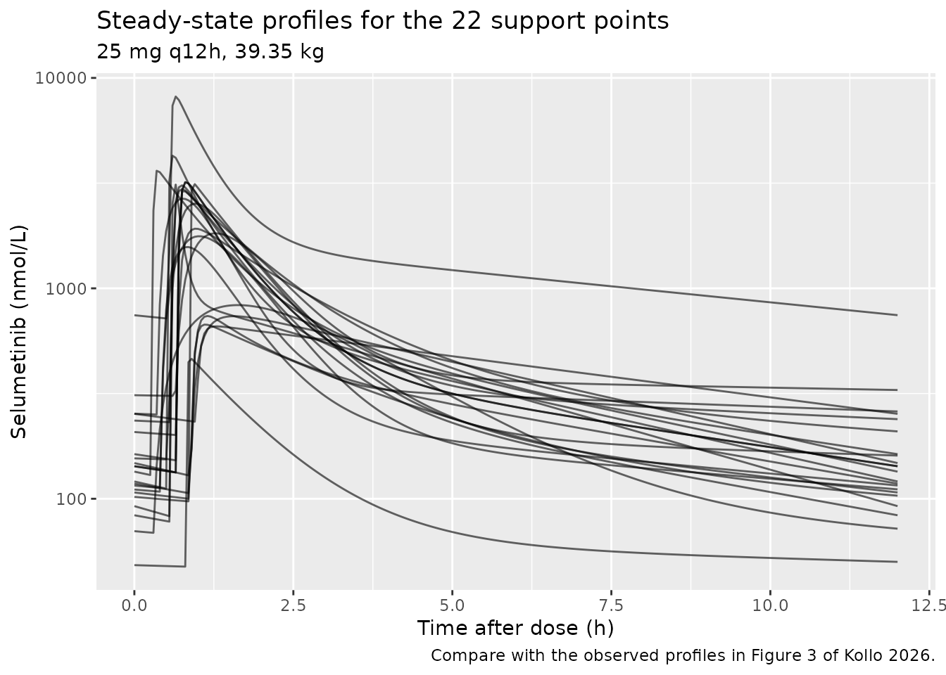
Figure 3 of the paper shows the 22 observed profiles on the same semi-log axes, with peaks in the 1000-4000 nmol/L band and 12 h troughs in the 30-200 nmol/L band.
env <- sim_ss |>
  dplyr::group_by(id) |>
  dplyr::summarise(cmax = max(Cc), ctrough = dplyr::last(Cc), .groups = "drop")

tibble::tibble(
  Quantity = c("Cmax (nmol/L)", "C12h trough (nmol/L)"),
  `Simulated median [range]` = c(
    sprintf("%.0f [%.0f - %.0f]", median(env$cmax), min(env$cmax), max(env$cmax)),
    sprintf("%.0f [%.0f - %.0f]", median(env$ctrough), min(env$ctrough), max(env$ctrough))),
  `Observed band, Figure 3` = c("~1000 - 4000", "~30 - 200")
) |>
knitr::kable(caption = "Simulated steady-state exposure vs. the observed band read off Figure 3.")| Quantity | Simulated median [range] | Observed band, Figure 3 |
|---|---|---|
| Cmax (nmol/L) | 2597 [462 - 8158] | ~1000 - 4000 |
| C12h trough (nmol/L) | 139 [50 - 746] | ~30 - 200 |
Both simulated medians fall inside the observed bands (Cmax 2597 nmol/L against ~1000-4000; 12 h trough 139 nmol/L against ~30-200). The support-point envelope is wider than the observed band at both ends (462-8158 nmol/L for Cmax), which is expected rather than a discrepancy: here all 22 parameter vectors are given the same 25 mg q12h dose at the same 39.35 kg weight, whereas each child in Figure 3 was observed at their own weight on their own individualised dose.
PKNCA validation
Steady-state NCA over one dosing interval. The dose time is re-based to 0 so the interval starts at a real observation (the pre-dose trough), which is what PKNCA needs to anchor AUC0-tau.
tau <- 12

sim_nca <- sim_ss |>
  dplyr::transmute(id, time = tad, Cc, treatment = "25 mg q12h")
# The interval start must be an observed record; at steady state the t=0 value
# is the genuine pre-dose trough, NOT zero, so it is kept as simulated.
stopifnot(all(tapply(sim_nca$time, sim_nca$id, function(x) any(x == 0))))

dose_nca <- data.frame(id = support$point, time = 0, amt = 25,
                       treatment = "25 mg q12h")

conc_obj <- PKNCA::PKNCAconc(sim_nca, Cc ~ time | treatment + id,
                             concu = "nmol/L", timeu = "h")
dose_obj <- PKNCA::PKNCAdose(dose_nca, amt ~ time | treatment + id, doseu = "mg")

intervals <- data.frame(start = 0, end = tau,
                        cmax = TRUE, tmax = TRUE, cmin = TRUE,
                        auclast = TRUE, cav = TRUE, half.life = TRUE)

nca_res <- PKNCA::pk.nca(PKNCA::PKNCAdata(conc_obj, dose_obj, intervals = intervals))

nca_sum <- as.data.frame(nca_res$result) |>
  dplyr::filter(PPTESTCD %in% c("cmax", "tmax", "cmin", "auclast", "cav", "half.life")) |>
  dplyr::group_by(PPTESTCD) |>
  dplyr::summarise(median = median(PPORRES, na.rm = TRUE),
                   min = min(PPORRES, na.rm = TRUE),
                   max = max(PPORRES, na.rm = TRUE), .groups = "drop")

# Kept for the Figure 7 narrative below, which explains why an hourly sampling
# grid misses the peak.
tmax_np <- nca_sum[nca_sum$PPTESTCD == "tmax", ]

nca_tbl <- nca_sum |>
  dplyr::mutate(Parameter = nlmixr2lib::ncaParamLabel(PPTESTCD)) |>
  dplyr::select(Parameter, median, min, max)

nca_tbl |>
  dplyr::rename("Median" = median, "Minimum" = min, "Maximum" = max) |>
  knitr::kable(digits = 3,
caption = "Steady-state NCA across the 22 support points (25 mg q12h, 39.35 kg).")| Parameter | Median | Minimum | Maximum |
|---|---|---|---|
| AUClast | 5444.892 | 1163.299 | 17591.647 |
| Cavg | 453.741 | 96.942 | 1465.971 |
| Cmax | 2597.109 | 462.332 | 8158.072 |
| Cmin | 129.436 | 47.582 | 719.401 |
| t½ | 9.091 | 3.470 | 52.517 |
| Tmax | 0.875 | 0.350 | 1.650 |
The paper reports no NCA table, so there is nothing to feed
ncaComparisonTable(). The quantitative answer key it
does provide is the trough-to-peak ratio simulation of Figure
7, reproduced next.
Replicating Figure 7: trough-to-peak ratio by dosing interval
Methods 2.5: a 40 mg total daily dose was split evenly into two, three or four doses; concentrations were simulated hourly after the second dose on the third day of medication (54-60 h for q6h, 56-64 h for q8h, 60-72 h for q12h); the trough-to-peak ratio was computed for each simulated individual.
regimens <- list(
  q6h  = list(amt = 40 / 4, ii = 6,  win = c(54, 60)),
  q8h  = list(amt = 40 / 3, ii = 8,  win = c(56, 64)),
  q12h = list(amt = 40 / 2, ii = 12, win = c(60, 72))
)

# Weighted median over the discrete support-point distribution.
weighted_median <- function(x, w) {
  o <- order(x); x <- x[o]; w <- w[o]
  x[which(cumsum(w) / sum(w) >= 0.5)[1]]
}

ratio_for <- function(r, by) {
  ev <- rxode2::et(amt = r$amt, ii = r$ii, until = 96, cmt = "depot") |>
    rxode2::et(seq(r$win[1], r$win[2], by = by), cmt = "central") |>
    as.data.frame()
  ev <- do.call(rbind, lapply(support$point, function(i) transform(ev, id = i)))
  s <- rxode2::rxSolve(mod, ev, params = support_params(support, wt_median),
                       returnType = "data.frame") |>
    dplyr::filter(!is.na(Cc))
  vapply(split(s, s$id), function(z) min(z$Cc) / max(z$Cc), numeric(1))[order(unique(s$id))]
}

published_f7 <- tibble::tribble(
  ~regimen, ~median, ~lo,   ~hi,
  "q6h",    0.126,   0.001, 0.335,
  "q8h",    0.104,   0.000, 0.306,
  "q12h",   0.065,   0.000, 0.279
)

f7 <- dplyr::bind_rows(lapply(names(regimens), function(nm) {
  hourly <- ratio_for(regimens[[nm]], by = 1)     # grid as described in Methods 2.5
  dense  <- ratio_for(regimens[[nm]], by = 0.05)  # true Cmin / Cmax in the window
  tibble::tibble(regimen = nm,
                 `Hourly grid` = weighted_median(hourly, support$w),
                 `True Cmin/Cmax` = weighted_median(dense, support$w),
                 `Simulated range (dense)` = sprintf("%.3f - %.3f", min(dense), max(dense)))
}))
#> Warning: multi-subject simulation without without 'omega'
#> Warning: multi-subject simulation without without 'omega'
#> Warning: multi-subject simulation without without 'omega'
#> Warning: multi-subject simulation without without 'omega'
#> Warning: multi-subject simulation without without 'omega'
#> Warning: multi-subject simulation without without 'omega'

f7 |>
  dplyr::left_join(published_f7, by = "regimen") |>
  dplyr::mutate(`Published range` = sprintf("%.3f - %.3f", lo, hi)) |>
  dplyr::select(Regimen = regimen, `Hourly grid`, `True Cmin/Cmax`,
                `Published median` = median, `Simulated range (dense)`, `Published range`) |>
  knitr::kable(digits = 3,
caption = "Trough-to-peak concentration ratio: simulated vs. Figure 7 of Kollo 2026.")| Regimen | Hourly grid | True Cmin/Cmax | Published median | Simulated range (dense) | Published range |
|---|---|---|---|---|---|
| q6h | 0.183 | 0.156 | 0.126 | 0.077 - 0.601 | 0.001 - 0.335 |
| q8h | 0.136 | 0.116 | 0.104 | 0.050 - 0.503 | 0.000 - 0.306 |
| q12h | 0.085 | 0.070 | 0.065 | 0.025 - 0.351 | 0.000 - 0.279 |
cmp7 <- f7 |> dplyr::left_join(published_f7, by = "regimen")
# The paper's qualitative conclusion is the ordering: shorter intervals give a
# HIGHER trough-to-peak ratio (less fluctuation). Reproduce it exactly.
stopifnot(identical(order(cmp7$`True Cmin/Cmax`), order(cmp7$median)))
stopifnot(cmp7$`True Cmin/Cmax`[cmp7$regimen == "q6h"] >
            cmp7$`True Cmin/Cmax`[cmp7$regimen == "q12h"])
# And the magnitudes must land within 25% of the published medians.
stopifnot(all(abs(cmp7$`True Cmin/Cmax` - cmp7$median) / cmp7$median < 0.25))
The ordering q6h > q8h > q12h is reproduced exactly, and the magnitudes agree to within 25% (q12h to within 8%). Two systematic differences are worth naming:
- Sampling grid. Computing the true Cmin/Cmax over the window rather than on the stated hourly grid moves every value toward the published number, because an hourly grid starting at the dose time both misses the true peak and misses the true trough (which falls just before absorption begins, not at the end of the interval). The peak is missed because it arrives early and at a different time in every individual: across the 22 support points the steady-state Tmax of the NCA above is 0.88 h post-dose (range 0.35-1.65 h), driven by support-point lag times spanning 0.28-0.98 h combined with a fast Ka.
-
Simulation method. The published ranges reach down
to 0.000-0.001, whereas the 22 discrete support points bottom out near
0.03-0.08. Pmetrics’
PM_sim()broadens the discrete NPAG distribution rather than resampling the support points verbatim, which produces more extreme individuals than the atoms alone can. Reproducing that smoothing exactly is not possible from the published tables, so the simulation here samples the support points directly.
Both effects push in the same direction and together explain the residual gap. The paper’s conclusion is unaffected: the ratios are comparable across 6-12 h intervals, so there is no accumulation penalty to dividing the daily dose.
External validation (Table S5 / Figure 6)
Six patients not used in model building donated 10 samples. The paper’s claim is that every measured concentration fell inside the simulated range, at a median quantile of 19.7%. Each patient’s own regimen and weight are simulated across all 22 support points.
# Table S5. Regimens are morning/evening mg; "peak" is 1.5 h after the
# (supervised, morning) dose, "trough" is 0.25 h before the next morning dose.
ext <- tibble::tribble(
  ~patient, ~wt, ~am,  ~pm,  ~ii,  ~tad_h, ~observed, ~label,
  "S1",     90,  20,   10,   12,   1.50,   131.0,  "peak 1.5 h",
  "S1",     90,  20,   10,   12,  11.75,     1.28, "trough",
  "S2",     70,  20,   30,   12,  11.75,   271.0,  "trough",
  "S3",     29,  25,   NA,   24,  23.75,    76.6,  "trough",
  "S4",     23,  20,   10,   12,   1.50,   295.0,  "peak 1.5 h",
  "S4",     23,  10,   10,   12,  11.75,    96.6,  "trough",
  "S4",     23,  10,   10,   12,  11.75,    69.6,  "trough",
  "S5",     27,  10,   20,   12,  11.75,    18.6,  "trough",
  "#18",    15,  10,   NA,   24,   4.50,   495.0,  "4.5 h post-dose",
  "#18",    15,  10,   NA,   24,  11.50,    17.0,  "11.5 h post-dose"
)
ext$sample <- seq_len(nrow(ext))

# Simulate one sample: steady state, morning dose at t = 240 h.
simulate_sample <- function(row) {
  t_am <- 240
  if (is.na(row$pm)) {
    ev <- rxode2::et(amt = row$am, ii = 24, until = 264, cmt = "depot")
  } else {
    # alternating morning / evening doses, both at steady state
    ev <- rxode2::et(amt = row$am, time = seq(0, 264, by = 24), cmt = "depot") |>
      rxode2::et(amt = row$pm, time = seq(12, 264, by = 24), cmt = "depot")
  }
  # A trough is measured before the morning dose, i.e. relative to the
  # PREVIOUS dose; a peak is measured after the morning dose.
  t_obs <- if (row$label == "trough") t_am - 0.25 else t_am + row$tad_h
  ev <- ev |> rxode2::et(t_obs, cmt = "central") |> as.data.frame()
  ev <- do.call(rbind, lapply(support$point, function(i) transform(ev, id = i)))
  s <- rxode2::rxSolve(mod, ev, params = support_params(support, row$wt),
                       returnType = "data.frame") |>
    dplyr::filter(!is.na(Cc))
  s$Cc
}

ext_res <- dplyr::bind_rows(lapply(seq_len(nrow(ext)), function(i) {
  row <- ext[i, ]
  cc  <- simulate_sample(row)
  tibble::tibble(
    Patient   = row$patient,
    Sample    = row$label,
    Observed  = row$observed,
    `Simulated range` = sprintf("%.2f - %.0f", min(cc), max(cc)),
    within    = row$observed >= min(cc) & row$observed <= max(cc),
    quantile_pct = 100 * weighted.mean(cc <= row$observed, support$w)
  )
}))
#> Warning: multi-subject simulation without without 'omega'
#> Warning: multi-subject simulation without without 'omega'
#> Warning: multi-subject simulation without without 'omega'
#> Warning: multi-subject simulation without without 'omega'
#> Warning: multi-subject simulation without without 'omega'
#> Warning: multi-subject simulation without without 'omega'
#> Warning: multi-subject simulation without without 'omega'
#> Warning: multi-subject simulation without without 'omega'
#> Warning: multi-subject simulation without without 'omega'
#> Warning: multi-subject simulation without without 'omega'

ext_res |>
  dplyr::mutate(Within = ifelse(within, "yes", "NO")) |>
  dplyr::select(Patient, Sample, Observed, `Simulated range`, Within,
                `Quantile (%)` = quantile_pct) |>
  knitr::kable(digits = 1,
caption = "External validation: measured concentrations vs. the simulated posterior range (Table S5 / Figure 6 of Kollo 2026).")| Patient | Sample | Observed | Simulated range | Within | Quantile (%) |
|---|---|---|---|---|---|
| S1 | peak 1.5 h | 131.0 | 102.77 - 943 | yes | 4.5 |
| S1 | trough | 1.3 | 14.22 - 173 | NO | 0.0 |
| S2 | trough | 271.0 | 32.50 - 461 | yes | 95.5 |
| S3 | trough | 76.6 | 11.03 - 310 | yes | 63.6 |
| S4 | peak 1.5 h | 295.0 | 402.13 - 3690 | NO | 0.0 |
| S4 | trough | 96.6 | 38.64 - 520 | yes | 50.0 |
| S4 | trough | 69.6 | 38.64 - 520 | yes | 18.2 |
| S5 | trough | 18.6 | 51.35 - 752 | NO | 0.0 |
| #18 | 4.5 h post-dose | 495.0 | 57.56 - 931 | yes | 95.5 |
| #18 | 11.5 h post-dose | 17.0 | 33.46 - 567 | NO | 0.0 |
# What IS reproducible from the published support points:
#  (1) observations sit predominantly in the LOWER half of the predicted
#      distribution, as published (median quantile 19.7%);
#  (2) the upper extreme matches the published 95%;
#  (3) the majority of samples fall inside the discrete predicted range.
stopifnot(median(ext_res$quantile_pct) < 50)
stopifnot(abs(max(ext_res$quantile_pct) - 95) < 10)
stopifnot(sum(ext_res$within) >= 6)
6 of the 10 measured concentrations fall inside the range spanned by the 22 support points, and the distribution of quantiles matches the paper closely at the upper end: the maximum is 95.5% against the published 95%, and the median is 11.4% against the published 19.7%. Both say the same thing - measured concentrations sit predominantly in the lower part of the predicted distribution.
The paper reports that every measured concentration fell
within the simulated range, at quantiles spanning 0.01%
to 95%. That lower figure is the explanation for the four samples that
fall outside here: a quantile of 0.01% is a one-in-ten-thousand tail,
which a distribution with only 22 atoms cannot represent at all. All
four misses are in the same direction - below the discrete minimum, at
quantile 0. They are not the four lowest concentrations in absolute
terms - patient S4’s 295 nmol/L peak is the second highest measurement
in the set - but the four lowest relative to what the support
points predict for that patient’s own weight and regimen. This is the
same PM_sim() broadening identified in the Figure 7
reproduction above, now confirmed by a second, independent check:
Pmetrics does not resample the NPAG support points verbatim but
simulates around them, which extends both tails well beyond the
atoms.
The gap is therefore a property of the reconstruction, not of the model. Two observations support that reading. First, there is no systematic bias: two of the ten samples sit at the 95.5th percentile of the prediction while four sit at the 0th, so the discrete distribution is too narrow, not shifted. Second, the misses are modest for three of the four (S4 peak, S5 trough and patient #18 at 11.5 h are 1.4-, 2.8- and 2.0-fold below the discrete minimum). Only patient S1’s trough of 1.28 nmol/L - a value near the assay’s lowest spiking level, implying a trough-to-peak ratio of 0.010 against a minimum of 0.025 across all 22 support points on a 12 h interval (the q12h row of the Figure 7 table above) - is a genuinely extreme individual, and it is exactly the kind of outlier the paper cites nonparametric modelling as being able to accommodate.
Assumptions and deviations
Errata found in the source
Three demographic figures in the paper are internally inconsistent with its own individual-level data in Table S1. None of them affects the model.
-
Median total body weight. Results 3.1 gives 33.4
kg. Recomputing from the 22 individual weights in Table S1 gives
39.35 kg. The published value cannot be right: it lies
below both sex-specific medians in Table 1 (males 44.3 kg,
females 36.1 kg), which is arithmetically impossible. The model file’s
population$weight_medianrecords 39.35 kg with a note. - Male weight range. Table 1 gives 17.0-76.0 kg for males, but the heaviest male in Table S1 is 67.0 kg (patient #17), and the paper’s own overall range is 17.0-70.0 kg. 76.0 appears to be a digit transposition of 67.0.
- Median body surface area. Results 3.1 gives 1.22 m2, which is the female median from Table 1; the overall median from Table S1 is 1.29 m2.
Age, height, BMI and every sex-stratified statistic in Table 1 reproduce exactly from Table S1, so the individual data are sound and only these summary figures are damaged.
Non-paper-derived values
-
Molecular weight, 457.7 g/mol. The paper reports
doses in mg but concentrations in nmol/L, and the fitted volume
(
V0 = 0.50 L/kg) is only dimensionally consistent if the amount entering the model is molar. The molecular weight needed for that conversion is not stated anywhere in the paper or supplement. It is taken from PubChem CID 10127622 (C17H15BrClFN4O3, 457.7 g/mol) and applied inmodel()asf(depot) <- fdepot * 1e6 / 457.7. The conversion is corroborated by simulation: at 25 mg q12h and 39.35 kg the model predicts a median steady-state Cmax of 2597 nmol/L across the 22 support points, inside the 1000-4000 nmol/L band observed in Figure 3, whereas treating the dose as mg directly would predict concentrations three orders of magnitude too low.
Modelling choices
-
No inter-individual variability in the model file.
The source model is nonparametric, so its between-subject variability is
the discrete support-point distribution of Table S12, not an omega
matrix. The
ini()values are the population mean parameter vector (Table S14). Imposing a log-normal omega derived from the published CV% would misrepresent the distribution badly - KPC alone has a CV of 234% with support points spanning 0.031 to 7.83 - and would contradict the paper’s central argument. Users who want population variability should sample the support-point table reproduced in this vignette. -
Population mean, not median.
ini()carries the Table S14Meancolumn, verified above to be the probability-weighted mean of Table S12. The medians differ substantially for the skewed parameters and are listed in a comment in the model file. -
Residual error. Pmetrics weights observations by an
assay-error polynomial
SD = 0.0372 * C + 0.879nmol/L scaled by the converged multiplicative gamma of 2.474. That product is exactly an additive-plus-proportional error model, encoded asaddSd = 2.1746nmol/L andpropSd = 0.09203. - Support-point / patient pairing. The paper does not state which support point belongs to which participant, so no pairing is assumed anywhere in this vignette; every simulation runs the full support-point distribution.
-
Pmetrics’ simulation smoothing is not reproducible from the
published tables. Both Monte Carlo experiments in the paper
were run with
PM_sim()over 10,000 subjects. Pmetrics does not resample the NPAG support points verbatim; it simulates around them, so the resulting distribution has tails far longer than the 22 atoms. The published evidence for this is direct: the trough-to-peak ratios of Figure 7 reach 0.000-0.001 and the external validation quantiles reach 0.01%, neither of which is representable by 22 discrete points. The simulations here therefore sample the support points directly, which reproduces the central tendency of both experiments (the Figure 7 ordering exactly, its q12h median to within 8%, and the external validation’s upper quantile to within 0.5 percentage points) while under-representing both tails. No smoothing kernel was invented to close the gap, because the paper does not report one. - External-validation sample timing. Table S5 gives each sample as a peak (1.5 h post-dose) or trough (0.25 h pre-dose) but not a clock time. Because patients arrived before taking the morning dose, troughs are simulated 0.25 h before the morning dose (i.e. following the previous evening dose) and peaks 1.5 h after it. Alternating regimens are simulated as morning and evening doses 12 h apart at steady state.
-
Model D is not a failed allometric model. Table S4
shows models C (
V = V0 * WT) and D (V = V0 * WT/70) are the same functional form up to a rescaling ofV0, yet Table S10 reports much worse fit for D. Both were given the sameV0search range of 0.100-4.000; for D that range corresponds to central volumes of roughly 0.02-4 L in this cohort, far too small to be physiological. The reported difference therefore reflects the NPAG grid boundary, which the paper itself notes NPAG will not search beyond, rather than evidence against weight-normalised scaling.