Flurbiprofen (Kumpulainen 2010)
Source:vignettes/articles/Kumpulainen_2010_flurbiprofen.Rmd
Kumpulainen_2010_flurbiprofen.RmdModel and source
Citation: Kumpulainen E, Valitalo P, Kokki M, Lehtonen M, Hooker A, Ranta V-P, Kokki H. Plasma and cerebrospinal fluid pharmacokinetics of flurbiprofen in children. Br J Clin Pharmacol. 2010;70(4):557-566. doi:10.1111/j.1365-2125.2010.03720.x.
Description: Three-compartment population PK model with a separate cerebrospinal-fluid (CSF) compartment for flurbiprofen in 64 healthy children aged 3 months to 13 years (Kumpulainen 2010). Two parallel absorption routes: oral syrup via an absorption compartment with lag time (K12) and a single first-order ka, and IV flurbiprofen axetil prodrug via a separate dosing compartment that converts to flurbiprofen with a first-order rate constant (K42). Plasma kinetics scaled allometrically by weight (exponents fixed at 0.75 for CL and 1 for all volumes, including the CSF volume held fixed at 0.15 L/70 kg per literature). The paper’s QCSF + UPTK parameterisation is encoded as canonical influx / efflux clearances clin = QCSF * UPTK and clef = QCSF, with fraction unbound (fu) gating only the central-to-CSF flux.
Population
64 healthy children aged 3 months to 13 years (median 5.2 years; weight median 20 kg, range 7-76 kg) scheduled for elective lower-body surgery with spinal anaesthesia at Kuopio University Hospital, Finland (Kumpulainen 2010 Table 1). 37 received a single 1 mg/kg oral dose of flurbiprofen syrup (Froben, 5 mg/mL); 27 received a 10-min IV injection of 0.9 mg/kg flurbiprofen axetil (Ropion, 10 mg/mL) corresponding to approximately 0.65 mg/kg of flurbiprofen after in-vivo conversion by plasma esterases. 304 total plasma + 62 protein-free plasma + 60 total CSF flurbiprofen concentrations were modelled in NONMEM VI with first-order conditional estimation with interaction (FOCE-I).
Programmatic access to the structured population metadata is via
readModelDb("Kumpulainen_2010_flurbiprofen")()$population.
Source trace
Every ini() parameter carries an in-file source-trace
comment next to its value in
inst/modeldb/specificDrugs/Kumpulainen_2010_flurbiprofen.R.
The table below collects them in one place for review. All references
are to the final-model column of Kumpulainen 2010 Table 2 unless
noted.
| Equation / parameter | Value | Source location |
|---|---|---|
lka (K12, oral ka) |
5.5 1/h | Table 2: K12 = 5.5 (RSE 0.24) |
lka2 (K42, axetil conversion) |
29 1/h | Table 2: K42 = 29 (RSE 0.32), half-life ~1.4 min |
ltlag (oral lag time) |
0.11 h | Table 2: lag time = 0.11 (RSE 0.16) = 6 min |
lcl (CL) |
0.96 L/h / 70 kg | Table 2: CL = 0.96 (RSE 0.057) |
lvc (V_central) |
3.6 L / 70 kg | Table 2: V (central) = 3.6 (RSE 0.11) |
lq (Q shallow peripheral) |
1.5 L/h | Table 2: Q (shallow peripheral, “Q2”) = 1.5 (RSE 0.39) |
lvp (V_shallow) |
1.8 L / 70 kg | Table 2: V (shallow peripheral) = 1.8 (RSE 0.20) |
lq2 (Q deep peripheral) |
0.18 L/h | Table 2: Q (deep peripheral) = 0.18 (RSE 0.30) |
lvp2 (V_deep) |
2.7 L / 70 kg | Table 2: V (deep peripheral) = 2.7 (RSE 0.18) |
lfdepot (oral F) |
0.81 | Table 2: bioavailability = 0.81 (RSE 0.055; bootstrap 0.71-0.91) |
lclin (= QCSF * UPTK) |
0.12 * 6.8 = 0.816 L/h | Table 2: QCSF = 0.12; UPTK = 6.8; see reparameterisation note below |
lclef (= QCSF) |
0.12 L/h | Table 2: QCSF = 0.12 (RSE 0.27) |
lvcsf (V_CSF, fixed) |
0.15 L / 70 kg | Results, popPK model: “The volume of the CSF compartment (0.15 l) was retrieved from the literature [13] and also scaled by weight” |
lfu (fraction unbound) |
0.00031 | Table 2: protein-free fraction = 0.00031 (RSE 0.043); = 0.031% per Results |
e_wt_cl (allometric CL) |
0.75 (fixed) | Table 2 footnote; Discussion: “the exponents were fixed to 1 and 0.75 in this study” |
e_wt_vc_vp (allometric volumes) |
1.0 (fixed) | Table 2 footnote; applied to V_central, V_shallow, V_deep, V_CSF |
etalcl (IIV on CL) |
omega = 0.28 (SD) | Table 2: omega_CL = 0.28 (RSE 0.20; bootstrap 0.22-0.34) |
etalvc (IIV on V_central) |
omega = 0.28 (SD) | Table 2: omega_Vd = 0.28 (RSE 0.25; bootstrap 0.19-0.35) |
etalka (IIV on K12) |
omega = 0.81 (SD) | Table 2: omega_K12 = 0.81 (RSE 0.40; bootstrap 0.42-1.4) |
etalfu (IIV on fu) |
omega = 0.30 (SD) | Table 2: omega_fu = 0.30 (RSE 0.28; bootstrap 0.19-0.36) |
propSd (plasma residual SD) |
0.13 | Table 2: sigma plasma = 0.13 (RSE 0.065) |
propSd_Cu (unbound residual) |
0.13 | Same as plasma per Methods: “Unbound observations were included in the same compartment as total plasma observations” |
propSd_Ccsf (CSF residual SD) |
0.50 | Table 2: sigma CSF = 0.50 (RSE 0.091) |
d/dt(central) (Figure 1 ODE) |
n/a | Figure 1 schematic + Methods modelling strategy |
d/dt(csf) (CSF kinetics) |
n/a | Figure 1 + Methods: K_central->CSF = (QCSF * UPTK * fu) / V_central; K_CSF->central = QCSF / V_CSF |
Virtual cohort
Original observed data are not publicly available. The figures below use a virtual paediatric cohort whose body-weight distribution approximates the paper’s reported median 20 kg with range 7-76 kg (Table 1). Half of the virtual subjects receive 1 mg/kg oral syrup; the other half receive 0.65 mg/kg of flurbiprofen-equivalent IV axetil (the depot2 compartment receives this mass directly; the in-vivo axetil-to-flurbiprofen conversion is captured by the model’s ka2 = K42 first-order kinetic).
set.seed(20100506L)  # Kumpulainen 2010 accepted date 6 May 2010 = 2010-05-06

n_per_arm <- 50L
ages_yr <- c(0.25, runif(n_per_arm - 2L, min = 0.5, max = 13), 13)
# Simple WHO-style weight-for-age approximation: kg ~ 8 + age*2 in the paediatric range,
# with mild log-normal noise to span the paper's observed 7-76 kg envelope.
wt_kg_typical <- 8 + 2 * ages_yr
weights_kg <- pmax(7, pmin(76,
  exp(log(wt_kg_typical) + rnorm(n_per_arm, sd = 0.20))
))

make_cohort <- function(arm, dose_mg_per_kg, cmt, weights_kg, id_offset = 0L) {
  ids <- id_offset + seq_along(weights_kg)
  doses <- tibble(
    id    = ids,
    time  = 0,
    amt   = dose_mg_per_kg * weights_kg,
    evid  = 1L,
    cmt   = cmt,
    WT    = weights_kg,
    arm   = arm
  )
  obs_times <- c(seq(0, 1, by = 0.05), seq(1.1, 6, by = 0.1), seq(6.5, 20, by = 0.5))
  obs <- tidyr::expand_grid(
    id   = ids,
    time = obs_times
  ) |>
    dplyr::left_join(doses |> dplyr::select(id, WT, arm), by = "id") |>
    dplyr::mutate(amt = NA_real_, evid = 0L, cmt = "Cc")
  dplyr::bind_rows(doses, obs) |>
    dplyr::arrange(id, time, dplyr::desc(evid))
}

events <- dplyr::bind_rows(
  make_cohort("oral 1 mg/kg",   1.00, "depot",  weights_kg, id_offset =   0L),
  make_cohort("IV 0.65 mg/kg",  0.65, "depot2", weights_kg, id_offset = 100L)
)
stopifnot(!anyDuplicated(unique(events[, c("id", "time", "evid")])))
Simulation
The figures below combine two simulations:
- A typical-value simulation for a 20 kg child to compare directly against the source paper’s “predicted Cmax / tmax for a typical 20 kg child” claims in Results, and
- A stochastic population simulation with the full random-effect structure for the VPC-style plots and the NCA validation.
typical_events <- dplyr::bind_rows(
  make_cohort("oral 1 mg/kg",   1.00, "depot",  rep(20, 1L), id_offset = 0L),
  make_cohort("IV 0.65 mg/kg",  0.65, "depot2", rep(20, 1L), id_offset = 100L)
)
mod_typical <- m |> rxode2::zeroRe()
#> ℹ parameter labels from comments will be replaced by 'label()'
sim_typical <- rxode2::rxSolve(mod_typical, events = typical_events,
                               keep = c("WT", "arm")) |>
  as.data.frame()
#> ℹ omega/sigma items treated as zero: 'etalcl', 'etalvc', 'etalka', 'etalfu'
#> Warning: multi-subject simulation without without 'omega'
sim <- rxode2::rxSolve(m, events = events, keep = c("WT", "arm")) |>
  as.data.frame()
#> ℹ parameter labels from comments will be replaced by 'label()'
Replicate published figures
Figure 3: total plasma, unbound plasma, and CSF concentration-time profiles
Kumpulainen 2010 Figure 3 shows raw observed concentration-time data
in four panels: (A) IV total plasma, (B) oral total plasma, (C) both
arms protein-free (unbound) plasma, (D) both arms total CSF. The panels
below show the stochastic-simulation median + 90% interval per arm for
each of the three modelled outputs (total plasma Cc,
unbound plasma Cu, CSF Ccsf).
plasma_summary <- sim |>
  group_by(arm, time) |>
  summarise(
    Q05 = quantile(Cc, 0.05, na.rm = TRUE),
    Q50 = quantile(Cc, 0.50, na.rm = TRUE),
    Q95 = quantile(Cc, 0.95, na.rm = TRUE),
    .groups = "drop"
  ) |>
  filter(time <= 6)

ggplot(plasma_summary, aes(time, Q50)) +
  geom_ribbon(aes(ymin = Q05, ymax = Q95), alpha = 0.25) +
  geom_line() +
  facet_wrap(~ arm) +
  labs(x = "Time (h)", y = "Total plasma flurbiprofen Cc (mg/L)",
       title = "Figure 3A-B equivalent: total plasma simulated profiles",
       caption = "Replicates Figure 3A (IV arm) and 3B (oral arm) of Kumpulainen 2010. Ribbon = 5%-95% percentile band over the simulated cohort.") +
  theme_bw()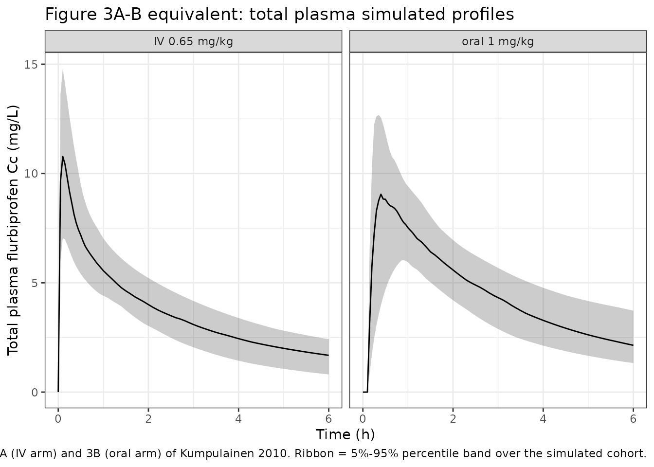
unbound_summary <- sim |>
  group_by(arm, time) |>
  summarise(
    Q05 = quantile(Cu * 1000, 0.05, na.rm = TRUE),
    Q50 = quantile(Cu * 1000, 0.50, na.rm = TRUE),
    Q95 = quantile(Cu * 1000, 0.95, na.rm = TRUE),
    .groups = "drop"
  ) |>
  filter(time <= 6)

ggplot(unbound_summary, aes(time, Q50)) +
  geom_ribbon(aes(ymin = Q05, ymax = Q95), alpha = 0.25) +
  geom_line() +
  facet_wrap(~ arm) +
  labs(x = "Time (h)", y = "Unbound plasma flurbiprofen Cu (ug/L)",
       title = "Figure 3C equivalent: unbound plasma simulated profiles",
       caption = "Replicates Figure 3C of Kumpulainen 2010. Cu = fu * Cc with fu = 0.00031.") +
  theme_bw()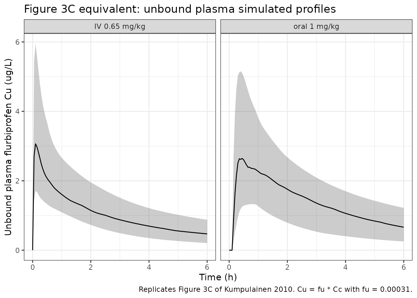
csf_summary <- sim |>
  group_by(arm, time) |>
  summarise(
    Q05 = quantile(Ccsf * 1000, 0.05, na.rm = TRUE),
    Q50 = quantile(Ccsf * 1000, 0.50, na.rm = TRUE),
    Q95 = quantile(Ccsf * 1000, 0.95, na.rm = TRUE),
    .groups = "drop"
  ) |>
  filter(time <= 6)

ggplot(csf_summary, aes(time, Q50)) +
  geom_ribbon(aes(ymin = Q05, ymax = Q95), alpha = 0.25) +
  geom_line() +
  facet_wrap(~ arm) +
  labs(x = "Time (h)", y = "Total CSF flurbiprofen Ccsf (ug/L)",
       title = "Figure 3D equivalent: total CSF simulated profiles",
       caption = "Replicates Figure 3D of Kumpulainen 2010. Median CSF Cmax 1-2 h post-dose.") +
  theme_bw()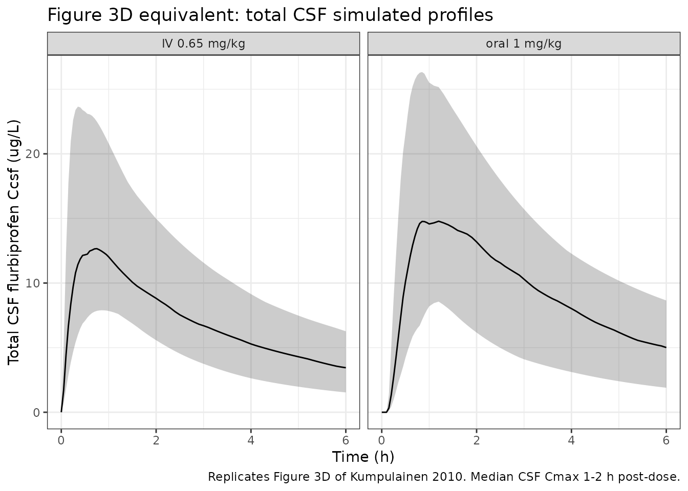
PKNCA validation
The source paper reports model-predicted Cmax and tmax for the three outputs in a typical 20 kg child receiving the standard 1 mg/kg oral dose (Cc and Ccsf) or 0.65 mg/kg IV (Ccsf only). PKNCA reproduces those summaries from the typical-value simulation. The remaining NCA parameters (AUC, t1/2) are reported here for completeness; the source paper does not publish reference values for them, so no Reference column is shown.
nca_for_output <- function(sim_df, conc_col, conc_unit, time_unit = "h") {
  conc <- sim_df |>
    dplyr::filter(!is.na(.data[[conc_col]])) |>
    dplyr::transmute(id = id, time = time, Cc = .data[[conc_col]], arm = arm)
  # Guarantee a t=0 row per (id, arm) so PKNCA can anchor AUC0-* (extravascular
  # dosing -> Cc(0) = 0). Without this, the "Requesting an AUC range starting
  # (0) before the first measurement" warning fires for every subject.
  conc <- dplyr::bind_rows(
    conc,
    conc |> dplyr::distinct(id, arm) |> dplyr::mutate(time = 0, Cc = 0)
  ) |>
    dplyr::distinct(id, arm, time, .keep_all = TRUE) |>
    dplyr::arrange(id, arm, time)
  conc_obj <- PKNCA::PKNCAconc(conc, Cc ~ time | arm + id,
                               concu = conc_unit, timeu = time_unit)

  doses <- sim_df |>
    dplyr::group_by(id, arm) |>
    dplyr::slice_head(n = 1) |>
    dplyr::ungroup() |>
    dplyr::transmute(id = id, time = 0, amt = WT * dplyr::if_else(arm == "oral 1 mg/kg", 1.00, 0.65),
                     arm = arm)
  dose_obj <- PKNCA::PKNCAdose(doses, amt ~ time | arm + id, doseu = "mg")

  intervals <- data.frame(
    start       = 0,
    end         = Inf,
    cmax        = TRUE,
    tmax        = TRUE,
    aucinf.obs  = TRUE,
    half.life   = TRUE
  )
  PKNCA::pk.nca(PKNCA::PKNCAdata(conc_obj, dose_obj, intervals = intervals))
}
# Typical-value (1 child per arm) NCA: directly comparable to paper's Cmax/tmax
nca_typ_Cc   <- nca_for_output(sim_typical, "Cc",   "mg/L")
nca_typ_Ccsf <- nca_for_output(sim_typical, "Ccsf", "mg/L")
# Population NCA: medians across the virtual cohort, for completeness
nca_pop_Cc   <- nca_for_output(sim, "Cc",   "mg/L")
nca_pop_Ccsf <- nca_for_output(sim, "Ccsf", "mg/L")
Comparison against published predicted Cmax / tmax (typical 20 kg child)
Kumpulainen 2010 Results state, for a 20 kg child:
- Oral 1 mg/kg: “the predicted tmax was 27 min and Cmax 10 mg/L” (Cc).
- Oral 1 mg/kg: “model-predicted CSF Cmax and tmax after oral dosing (1 mg/kg) were 17 ug/L and 60 min, respectively”.
- IV 0.65 mg/kg: “model-predicted Cmax and tmax for CSF concentrations after i.v. injection (0.65 mg/kg) in a typical 20 kg child were 14 ug/L and 40 min, respectively”.
# Pull the typical-value Cmax/tmax for each (arm, output) into a long table
typ_results <- function(nca_res, output_label, scale = 1) {
  res <- as.data.frame(nca_res$result) |>
    dplyr::filter(PPTESTCD %in% c("cmax", "tmax")) |>
    dplyr::transmute(arm = arm, PPTESTCD = PPTESTCD,
                     PPORRES = PPORRES * dplyr::if_else(PPTESTCD == "cmax", scale, 1)) |>
    dplyr::mutate(output = output_label)
  res
}

simulated_long <- dplyr::bind_rows(
  typ_results(nca_typ_Cc,   "Cc (mg/L)"),
  typ_results(nca_typ_Ccsf, "Ccsf (ug/L)", scale = 1000)
)

# Paper-reported published values (Cmax in matching units, tmax in h)
published_typ <- tibble::tribble(
  ~arm,            ~output,        ~cmax, ~tmax,
  "oral 1 mg/kg",  "Cc (mg/L)",      10,   27/60,
  "oral 1 mg/kg",  "Ccsf (ug/L)",    17,   60/60,
  "IV 0.65 mg/kg", "Ccsf (ug/L)",    14,   40/60
)

# Build a comparison table per output
sim_table_long <- simulated_long |>
  dplyr::transmute(arm = arm, output = output, PPTESTCD = PPTESTCD, PPORRES = PPORRES)

comparison_tables <- lapply(unique(published_typ$output), function(out) {
  pub <- published_typ |> dplyr::filter(output == out) |>
    dplyr::select(arm, cmax, tmax)
  sim <- sim_table_long |> dplyr::filter(output == out) |>
    dplyr::select(arm, PPTESTCD, PPORRES)
  tbl <- nlmixr2lib::ncaComparisonTable(
    simulated = sim,
    reference = pub,
    by        = "arm",
    units     = c(cmax = if (out == "Cc (mg/L)") "mg/L" else "ug/L",
                  tmax = "h"),
    tolerance_pct = 20
  )
  cbind(`Output` = out, tbl)
})

comparison_tbl <- do.call(rbind, comparison_tables)

knitr::kable(
  comparison_tbl,
  caption = "Simulated (typical 20 kg child, zero random effects) vs Kumpulainen 2010 Results-section predicted Cmax / tmax. * differs from reference by more than +/- 20%.",
  align = c("l", "l", "l", "r", "r", "r")
)| Output | NCA parameter | arm | Reference | Simulated | % diff |
|---|---|---|---|---|---|
| Cc (mg/L) | Cmax (mg/L) | oral 1 mg/kg | 10 | 9.62 | -3.8% |
| Cc (mg/L) | Tmax (h) | oral 1 mg/kg | 0.45 | 0.5 | +11.1% |
| Ccsf (ug/L) | Cmax (ug/L) | oral 1 mg/kg | 17 | 16.4 | -3.3% |
| Ccsf (ug/L) | Cmax (ug/L) | IV 0.65 mg/kg | 14 | 13.7 | -2.5% |
| Ccsf (ug/L) | Tmax (h) | oral 1 mg/kg | 1 | 1 | +0.0% |
| Ccsf (ug/L) | Tmax (h) | IV 0.65 mg/kg | 0.667 | 0.7 | +5.0% |
Population-cohort NCA summary (no published reference values)
The remaining NCA parameters (AUC, t1/2) over the simulated cohort are reported here for context; the source paper does not publish reference values for them, so no Reference column is shown.
pop_summary <- function(nca_res, output_label, scale = 1) {
  as.data.frame(nca_res$result) |>
    dplyr::filter(PPTESTCD %in% c("aucinf.obs", "half.life")) |>
    dplyr::group_by(arm, PPTESTCD) |>
    dplyr::summarise(
      median = stats::median(PPORRES, na.rm = TRUE),
      q05    = stats::quantile(PPORRES, 0.05, na.rm = TRUE),
      q95    = stats::quantile(PPORRES, 0.95, na.rm = TRUE),
      .groups = "drop"
    ) |>
    dplyr::mutate(parameter = dplyr::recode(PPTESTCD,
                                            aucinf.obs = "AUC0-Inf (obs)",
                                            half.life  = "t1/2"),
                  output = output_label) |>
    dplyr::select(output, arm, parameter, median, q05, q95)
}

pop_table <- dplyr::bind_rows(
  pop_summary(nca_pop_Cc,   "Cc (mg/L)"),
  pop_summary(nca_pop_Ccsf, "Ccsf (ug/L)")
) |>
  dplyr::mutate(across(c(median, q05, q95), ~ signif(.x, 3)))

pop_table |>
  dplyr::rename(
    "Output"         = output,
    "Arm"            = arm,
    "NCA parameter"  = parameter,
    "Median"         = median,
    "5% percentile"  = q05,
    "95% percentile" = q95
  ) |>
  knitr::kable(
  caption = "Population-cohort median and 5%-95% range for AUC0-Inf and t1/2 (per arm and per output). No published reference values.",
  align = c("l", "l", "l", "r", "r", "r")
)| Output | Arm | NCA parameter | Median | 5% percentile | 95% percentile |
|---|---|---|---|---|---|
| Cc (mg/L) | IV 0.65 mg/kg | AUC0-Inf (obs) | 33.9000 | 21.3000 | 52.200 |
| Cc (mg/L) | IV 0.65 mg/kg | t1/2 | 5.4600 | 3.9000 | 8.120 |
| Cc (mg/L) | oral 1 mg/kg | AUC0-Inf (obs) | 42.1000 | 26.0000 | 76.000 |
| Cc (mg/L) | oral 1 mg/kg | t1/2 | 5.6700 | 3.7100 | 8.980 |
| Ccsf (ug/L) | IV 0.65 mg/kg | AUC0-Inf (obs) | 0.0651 | 0.0358 | 0.121 |
| Ccsf (ug/L) | IV 0.65 mg/kg | t1/2 | 5.4500 | 3.9000 | 8.050 |
| Ccsf (ug/L) | oral 1 mg/kg | AUC0-Inf (obs) | 0.0958 | 0.0362 | 0.163 |
| Ccsf (ug/L) | oral 1 mg/kg | t1/2 | 5.6600 | 3.7200 | 8.970 |
Assumptions and deviations
-
QCSF + UPTK reparameterised as clin + clef.
Kumpulainen 2010 Figure 1 / Methods write the central-to-CSF transfer
rate as
K_central_to_CSF = (QCSF * UPTK * fu) / V_central, with the CSF-to-central return rateK_CSF_to_central = QCSF / V_CSF. UPTK is dimensionless (estimated as 6.8 with bootstrap 95% CI 6.0-7.7). The packaged model preserves all numerical content but encodes this as the canonical Campagne 2019clin/clefpair:clin = QCSF * UPTK(CSF influx clearance applied to the unbound plasma concentrationfu * Cc) andclef = QCSF(CSF efflux clearance applied toCcsf). The uptake ratioUPTK = clin / clef = 6.8is recoverable post-hoc; in-file source-trace comments ininst/modeldb/specificDrugs/Kumpulainen_2010_flurbiprofen.Rdocument both the paper’s UPTK = 6.8 and QCSF = 0.12 L/h values. -
CSF volume held fixed at 0.15 L / 70 kg.
Kumpulainen 2010 Results, popPK section: “The volume of the CSF
compartment (0.15 l) was retrieved from the literature [13] and also
scaled by weight.”
lvcsfis wrapped infixed()to preserve this provenance. - Allometric exponents fixed at 0.75 (CL) and 1 (volumes). The paper estimated both exponents (0.774 and 1.01) and noted close agreement with the canonical values “the exponents were fixed to 1 and 0.75 in this study”. The shared volume exponent applies to V_central, V_shallow, V_deep, and V_CSF; the intercompartmental clearances Q2 (shallow), Q (deep), and QCSF carry no allometric scaling in Table 2 (the (WT/70) annotation appears only on CL and the four V rows).
-
BSV omega values are SDs of eta on the log scale.
The paper’s Table 2 reports omega values consistent with the
Results-section claim of “roughly 30% CV” inter-individual variability;
the omega for K12 (0.81) likewise aligns with “the inter-individual
variability for the oral absorption rate constant was estimated at 80%”.
The internal nlmixr2 variance is therefore
(paper omega)^2(0.28^2 = 0.0784 for CL, V, and Vd; 0.81^2 = 0.6561 for K12; 0.30^2 = 0.09 for fu). - IIV on volume applies to V_central only. The paper states “BSV was assigned to volume of distribution, clearance, oral absorption rate and fraction unbound” – a single omega is reported for “Vd” in Table 2. This is interpreted as IIV on the central volume V_central; the peripheral and CSF volumes carry no IIV.
-
Plasma sigma shared between total and unbound
observations. The paper reports two residual variances (plasma
and CSF), and writes Methods: “Unbound observations were included in the
same compartment as total plasma observations. They were defined as
special cases of total plasma observations”. The packaged model has
three outputs (
Cc,Cu,Ccsf) because nlmixr2 requires per-output residual-error parameters;propSd(Cc) andpropSd_Cu(Cu) carry the same source value of 0.13 to preserve this constraint. - IV axetil dosing convention. The paper reports the IV dose as 0.9 mg/kg of flurbiprofen axetil prodrug, which corresponds to approximately 0.65 mg/kg of flurbiprofen on a mass-equivalent basis. The packaged model assumes the user supplies the flurbiprofen-equivalent mass directly to the depot2 compartment; the K42 = 29 1/h conversion-rate constant then describes the in-vivo axetil-to-flurbiprofen hydrolysis. The 10-min IV infusion duration is short relative to K42’s half-life (1.4 min) and is captured by modelling the IV dose as an instantaneous bolus into depot2.
- Virtual cohort weight distribution. Original Table 1 weight values are not publicly available. The vignette uses a simple weight-for-age envelope (kg ~ 8 + 2 * age_years, with mild log-normal noise) to span the paper’s median 20 kg and range 7-76 kg envelope; this is good enough for typical-value Cmax / tmax replication but is not a high-fidelity match of the trial’s actual paediatric weight distribution.
- No NCA reference values for AUC or t1/2. The paper does not report population NCA summaries for AUC or terminal half-life, so the population-cohort summary table omits a Reference column for those parameters; only the typical-value Cmax / tmax claims in the Results section are validated against the simulation.
-
Race / ethnicity not modelled. Single-centre
Finnish paediatric cohort; race / ethnicity was not reported in the
source paper, so the
populationmetadata records “Not reported” and the model carries no race covariate effects.