Remimazolam (Chen 2024)
Source:vignettes/articles/Chen_2024_remimazolam.Rmd
Chen_2024_remimazolam.RmdModel and source
- Citation: Chen Y, Gong C, Liu F, Jiao Z, Zheng X. Toward Model-Informed Precision Dosing for Remimazolam: A Population Pharmacokinetic-Pharmacodynamic Analysis. Pharmaceutics. 2024;16(9):1122. doi:10.3390/pharmaceutics16091122
- Description: Joint population PK/PD model for remimazolam, its inactive metabolite CNS 7054, and the bispectral index (BIS) in healthy Chinese adult volunteers (Chen 2024). Remimazolam is described by a three-compartment model with first-order elimination; the whole of parent clearance feeds a single transit compartment that delays the appearance of CNS 7054, which is itself described by a two-compartment model. Sedation is described by an effect compartment equilibrating with remimazolam plasma concentration and driving an inhibitory sigmoid Imax model on BIS. Body weight enters every clearance and volume term by allometric scaling with fixed exponents (0.75 and 1) and a 60 kg reference weight; no other covariate was retained on either the PK or the PD.
- Article: https://doi.org/10.3390/pharmaceutics16091122
Chen 2024 is a joint population PK/PD analysis of remimazolam, its inactive carboxylic-acid metabolite CNS 7054, and the bispectral index (BIS) in healthy Chinese adult volunteers. The paper packages three linked sub-models into a single structure (Figure 1):
- a three-compartment disposition model for remimazolam, dosed intravenously into the central compartment;
- a single transit compartment that delays the appearance of CNS 7054, fed by the whole of remimazolam clearance, followed by a two-compartment disposition model for CNS 7054;
- an effect compartment equilibrating with remimazolam plasma concentration and driving an inhibitory sigmoid Imax model on BIS.
Because the three sub-models are coupled (the metabolite is fed by parent clearance, and the effect compartment is driven by parent concentration) and were ultimately estimated simultaneously, they are packaged as a single model file rather than three.
Population
The model was fit to 55 healthy adult volunteers enrolled in a single-centre, placebo-controlled, randomised, dose-escalation clinical pharmacology study in China (ChiCTR1800015185 / ChiCTR1800015186); the analysis is a secondary analysis of that trial. Forty-six subjects received a single IV bolus of remimazolam at one of seven dose levels (0.025, 0.05, 0.075, 0.1, 0.2, 0.3, or 0.4 mg/kg) and nine received an IV bolus of 0.2 mg/kg over 1 min followed by a 1 mg/kg/h infusion for 2 h (Table 1).
The cohort was demographically narrow by design (Table 2): 40 men and 15 women (27.3 percent female), median age 28 years (range 19-43), median weight 62.5 kg (range 52-75), median height 167.5 cm (range 151-185), and BMI restricted by protocol to 19-24 kg/m2. The dataset comprised 1113 remimazolam plasma concentrations, 1206 CNS 7054 plasma concentrations, and 1026 BIS observations. Both analytes were assayed by LC/MS/MS over a 2-2000 ng/mL calibration range.
The authors screened age, height, and sex by stepwise forward
inclusion and backward elimination on both the PK and the PD parameters
and retained none of them, attributing the absence of
covariate effects to the homogeneity of the healthy-volunteer cohort.
Body weight enters only as fixed-exponent allometric scaling. The three
screened-but-not-retained covariates are recorded in the model file’s
covariatesDataExcluded metadata.
The same information is available programmatically via
readModelDb("Chen_2024_remimazolam")()$population.
Source trace
Every ini() entry in
inst/modeldb/specificDrugs/Chen_2024_remimazolam.R carries
an in-file comment pointing at its source location. They are collected
here for review.
| Equation / parameter | Value | Source location |
|---|---|---|
lcl (CLp) |
1.21 L/min | Table 3, CL for remimazolam (RSE 3%) |
lvc (V1) |
16 L | Table 3, V1 for remimazolam (RSE 8%) |
lvp (V2, shallow) |
22.6 L | Table 3, V2 for remimazolam (RSE 3%) |
lq (Q2) |
2.61 L/min | Table 3, Q2 for remimazolam (RSE 4%) |
lvp2 (V3, deep) |
23.5 L | Table 3, V3 for remimazolam (RSE 6%) |
lq2 (Q3) |
0.227 L/min | Table 3, Q3 for remimazolam (RSE 14%) |
lktr (Ktr) |
0.447 1/min | Table 3, Ktr for remimazolam (RSE 8%) |
lcl_cns7054 (CLm) |
0.0637 L/min | Table 3, CL for CNS7054 (RSE 3%) |
lvc_cns7054 (V5) |
3.72 L | Table 3, V5 for CNS7054 (RSE 5%) |
lq_cns7054 (Q4) |
0.166 L/min | Table 3, Q4 for CNS7054 (RSE 5%) |
lvp_cns7054 (V6) |
5.15 L | Table 3, V6 for CNS7054 (RSE 4%) |
lrbase (BIS_baseline) |
92.5 | Table 4 (RSE 1%) |
limax (Imax) |
54.5 BIS units | Table 4 (RSE 6%) |
lec50 (IC50) |
504 ng/mL | Table 4 (RSE 9%) |
lke0 (ke0) |
1.38 1/min | Table 4 (RSE 26%) |
lhill (Hill) |
1.44 | Table 4 (RSE 10%) |
e_wt_cl_q |
0.75 (fixed) | Equation (5), “values set to 0.75 for CL” |
e_wt_vc_vp |
1 (fixed) | Equation (5), “and 1 for volume” |
| Reference weight | 60 kg | Equation (5), printed denominator |
etalcl / etalvc / etalq /
etalvp / etalktr
|
20 / 55 / 24.3 / 32.1 / 40.1 % | Table 3, IIV block (remimazolam) |
etalcl_cns7054 / etalvc_cns7054 /
etalvp_cns7054
|
22.1 / 30.1 / 17.5 % | Table 3, IIV block (CNS 7054) |
etalimax / etalhill
|
27.2 / 48.8 % | Table 4 Cont., IIV block |
propSd |
23.2 % | Table 3, prop RUV for remimazolam |
propSd_cns7054 / addSd_cns7054
|
6.4 % / 43.13 ng/mL | Table 3, RUV block for CNS 7054 |
propSd_BIS |
11.2 % | Table 4 Cont., prop RUV pd |
| BSV model (exponential) | n/a | Equation (1) |
| RUV models (prop / add / combined) | n/a | Equations (2)-(4) |
| Allometric scaling | n/a | Equation (5) |
| Sigmoid Imax on BIS | n/a | Equation (8) (see Errata) |
| Compartment topology | n/a | Figure 1 schematic |
Virtual cohort
Original observed data are not publicly available. The simulations below use virtual populations whose weight distribution approximates the published trial demographics (median 62.5 kg, range 52-75 kg; Table 2) and whose dosing reproduces the two study arms of Table 1.
set.seed(20240826)

n_per_arm <- 40L

obs_times <- sort(unique(c(
  seq(0, 10, by = 0.5),
  seq(10, 60, by = 2),
  seq(60, 240, by = 5),
  seq(240, 720, by = 15)
)))

sample_wt <- function(n) {
  wt <- rnorm(n, mean = 62.5, sd = 5.5)
  pmin(pmax(wt, 52), 75)
}

# Arm 1 of Table 1: single IV bolus at one of seven dose levels.
make_bolus_arm <- function(dose_mgkg, n, id_offset) {
  subj <- tibble(
    id        = id_offset + seq_len(n),
    WT        = sample_wt(n),
    dose_mgkg = dose_mgkg,
    treatment = sprintf("%s mg/kg bolus", format(dose_mgkg, trim = TRUE))
  )
  doses <- subj |>
    mutate(time = 0, amt = dose_mgkg * WT, rate = 0, evid = 1L, cmt = "central")
  obs <- subj |>
    tidyr::crossing(time = obs_times) |>
    mutate(amt = NA_real_, rate = NA_real_, evid = 0L, cmt = "Cc")
  bind_rows(doses, obs) |> arrange(id, time, desc(evid))
}

bolus_levels <- c(0.025, 0.05, 0.075, 0.1, 0.2, 0.3, 0.4)

events <- bind_rows(lapply(seq_along(bolus_levels), function(i) {
  make_bolus_arm(bolus_levels[i], n_per_arm, id_offset = (i - 1L) * n_per_arm)
}))

# Arm 2 of Table 1: 0.2 mg/kg IV bolus over 1 min, then 1 mg/kg/h for 2 h.
inf_subj <- tibble(
  id        = 7L * n_per_arm + seq_len(n_per_arm),
  WT        = sample_wt(n_per_arm),
  dose_mgkg = NA_real_,
  treatment = "0.2 mg/kg over 1 min + 1 mg/kg/h x 2 h"
)
inf_doses <- bind_rows(
  inf_subj |> mutate(time = 0, amt = 0.2 * WT,     rate = 0.2 * WT,      evid = 1L, cmt = "central"),
  inf_subj |> mutate(time = 1, amt = 1 * WT * 2,   rate = 1 * WT / 60,   evid = 1L, cmt = "central")
)
inf_obs <- inf_subj |>
  tidyr::crossing(time = obs_times) |>
  mutate(amt = NA_real_, rate = NA_real_, evid = 0L, cmt = "Cc")

events <- bind_rows(events, inf_doses, inf_obs) |> arrange(id, time, desc(evid))

# Disjoint IDs across arms are mandatory: rxSolve keys subjects on id, and a
# collision silently merges two subjects into one that receives the summed dose.
stopifnot(!anyDuplicated(unique(events[, c("id", "time", "evid")])))
stopifnot(length(unique(events$id)) == 8L * n_per_arm)
Note the cmt = "Cc" on the observation rows. This model
declares three endpoints (Cc, Cc_cns7054,
BIS), so rxode2 builds a
dvid-to-cmt mapping in which the endpoints
occupy compartment slots after the seven ODE states;
observation records must therefore name an endpoint, not an ODE state.
This is the documented exception to the usual “point cmt at
the ODE state” rule, which applies to models with a single implicit
endpoint. rxode2 returns all three endpoints as columns at every
observation row regardless.
Simulation
mod <- readModelDb("Chen_2024_remimazolam")

sim <- rxode2::rxSolve(
  mod,
  events = events,
  keep   = c("WT", "treatment", "dose_mgkg"),
  # rxode2's automatic ODE-to-linCmt conversion corrupts the dvid mapping for
  # multi-output models with this many states.
  useLinCmt = FALSE
) |>
  as.data.frame()
#> ℹ parameter labels from comments will be replaced by 'label()'

stopifnot(length(unique(sim$id)) == 8L * n_per_arm)
stopifnot(!any(is.na(sim$Cc)), !any(is.na(sim$Cc_cns7054)), !any(is.na(sim$BIS)))
stopifnot(all(sim$Cc >= 0), all(sim$Cc_cns7054 >= 0))
Replicate published figures
Figure 3 - visual predictive checks
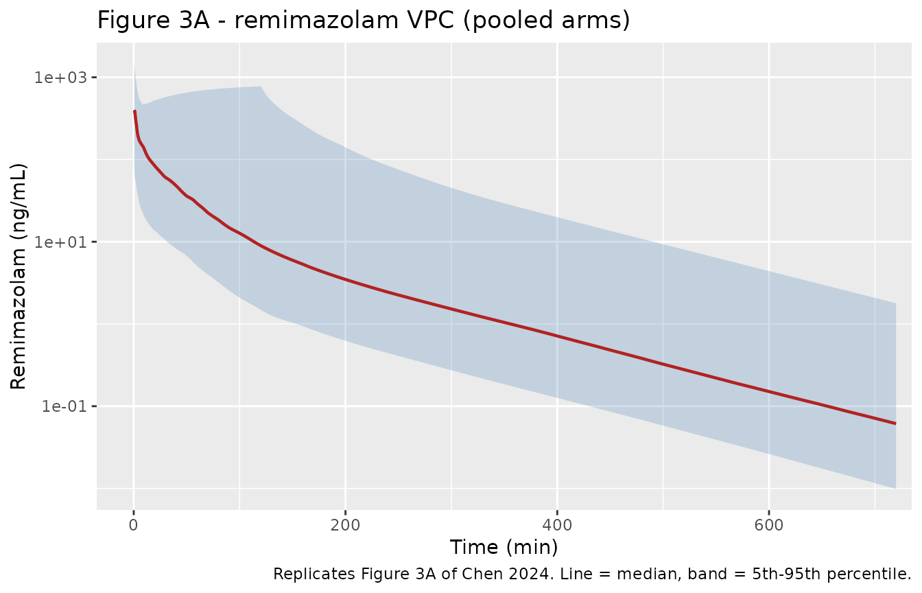
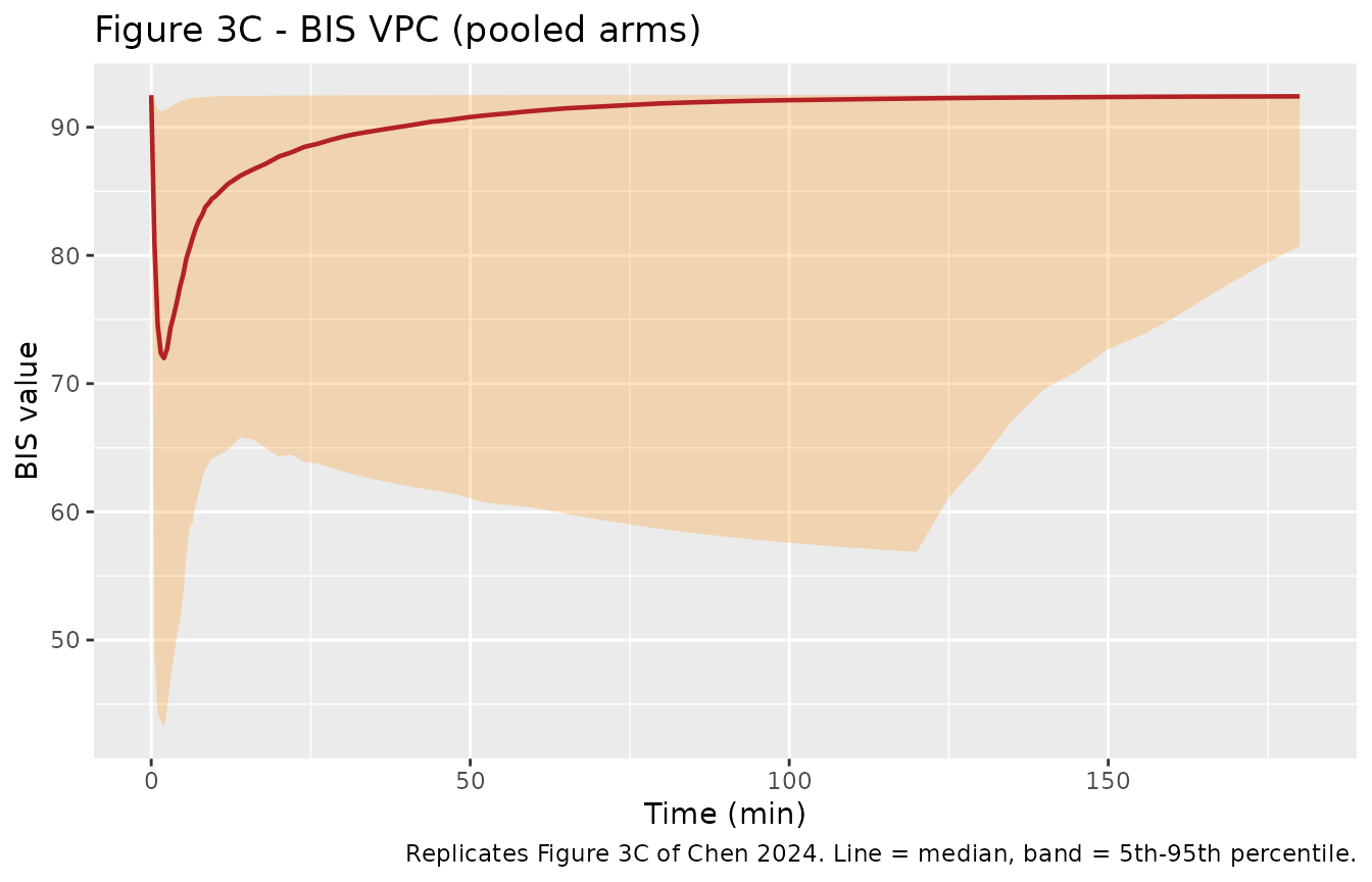
Chen 2024 Figure 3 shows VPCs for remimazolam (A, log scale), CNS 7054 (B, log scale), and BIS (C, linear scale). The panels below reproduce the same three views from the packaged model across the pooled study arms.
# Replicates Figure 3A of Chen 2024: remimazolam concentration, log scale.
sim |>
  filter(time > 0, Cc > 0) |>
  group_by(time) |>
  summarise(
    Q05 = quantile(Cc, 0.05), Q50 = quantile(Cc, 0.50), Q95 = quantile(Cc, 0.95),
    .groups = "drop"
  ) |>
  ggplot(aes(time, Q50)) +
  geom_ribbon(aes(ymin = Q05, ymax = Q95), alpha = 0.25, fill = "steelblue") +
  geom_line(colour = "firebrick", linewidth = 0.8) +
  scale_y_log10() +
  coord_cartesian(xlim = c(0, 700)) +
  labs(
    x = "Time (min)", y = "Remimazolam (ng/mL)",
    title = "Figure 3A - remimazolam VPC (pooled arms)",
    caption = "Replicates Figure 3A of Chen 2024. Line = median, band = 5th-95th percentile."
  )
# Replicates Figure 3B of Chen 2024: CNS 7054 concentration, log scale.
sim |>
  filter(time > 0, Cc_cns7054 > 0) |>
  group_by(time) |>
  summarise(
    Q05 = quantile(Cc_cns7054, 0.05), Q50 = quantile(Cc_cns7054, 0.50),
    Q95 = quantile(Cc_cns7054, 0.95), .groups = "drop"
  ) |>
  ggplot(aes(time, Q50)) +
  geom_ribbon(aes(ymin = Q05, ymax = Q95), alpha = 0.25, fill = "seagreen") +
  geom_line(colour = "firebrick", linewidth = 0.8) +
  scale_y_log10() +
  coord_cartesian(xlim = c(0, 700)) +
  labs(
    x = "Time (min)", y = "CNS 7054 (ng/mL)",
    title = "Figure 3B - CNS 7054 VPC (pooled arms)",
    caption = "Replicates Figure 3B of Chen 2024. Line = median, band = 5th-95th percentile."
  )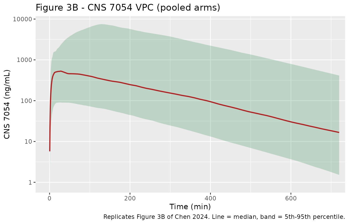
The metabolite peaks later and far higher than the parent and declines much more slowly, reproducing the qualitative shape of Figure 3B and the paper’s statement that remimazolam clearance exceeds CNS 7054 clearance by more than an order of magnitude.
# Replicates Figure 3C of Chen 2024: BIS, linear scale, first 180 min.
sim |>
  filter(time <= 180) |>
  group_by(time) |>
  summarise(
    Q05 = quantile(BIS, 0.05), Q50 = quantile(BIS, 0.50), Q95 = quantile(BIS, 0.95),
    .groups = "drop"
  ) |>
  ggplot(aes(time, Q50)) +
  geom_ribbon(aes(ymin = Q05, ymax = Q95), alpha = 0.25, fill = "darkorange") +
  geom_line(colour = "firebrick", linewidth = 0.8) +
  labs(
    x = "Time (min)", y = "BIS value",
    title = "Figure 3C - BIS VPC (pooled arms)",
    caption = "Replicates Figure 3C of Chen 2024. Line = median, band = 5th-95th percentile."
  )
Dose-response of sedation depth
sim |>
  filter(treatment != "0.2 mg/kg over 1 min + 1 mg/kg/h x 2 h", time <= 120) |>
  group_by(treatment, time) |>
  summarise(BIS = median(BIS), .groups = "drop") |>
  ggplot(aes(time, BIS, colour = treatment)) +
  geom_line(linewidth = 0.7) +
  geom_hline(yintercept = 92.5 - 54.5, linetype = "dashed", colour = "grey40") +
  labs(
    x = "Time (min)", y = "Median BIS",
    colour = "Dose group",
    title = "Median BIS by single-bolus dose level",
    caption = "Dashed line = BIS_baseline - Imax = 92.5 - 54.5 = 38, the model's maximum attainable suppression."
  )
Structural identity checks
For an IV bolus into the central compartment, this model implies three exact identities that jointly validate the units, the allometric scaling, and the 1:1 parent-to-metabolite amount transfer. They are checked here on a typical-value (no between-subject variability) subject weighing exactly 60 kg, which is the reference weight of Equation (5), so every parameter takes its published Table 3 value:
Cmax(remimazolam) = Dose / V1AUCinf(remimazolam) = Dose / CLp-
AUCinf(CNS 7054) = Dose / CLm(because all remimazolam is assumed to be converted to CNS 7054, the metabolite receives the entire dose)
typ_subj <- tibble(
  id        = seq_along(bolus_levels),
  WT        = 60,
  dose_mgkg = bolus_levels,
  treatment = sprintf("%s mg/kg bolus", format(bolus_levels, trim = TRUE))
)

typ_times <- sort(unique(c(seq(0, 20, by = 0.25), seq(20, 120, by = 1),
                           seq(120, 1440, by = 5))))

typ_events <- bind_rows(
  typ_subj |> mutate(time = 0, amt = dose_mgkg * WT, rate = 0, evid = 1L, cmt = "central"),
  typ_subj |> tidyr::crossing(time = typ_times) |>
    mutate(amt = NA_real_, rate = NA_real_, evid = 0L, cmt = "Cc")
) |>
  arrange(id, time, desc(evid))

sim_typical <- rxode2::rxSolve(
  rxode2::zeroRe(mod), events = typ_events,
  keep = c("WT", "treatment", "dose_mgkg"), useLinCmt = FALSE,
  omega = NA, sigma = NA
) |>
  as.data.frame()
#> ℹ parameter labels from comments will be replaced by 'label()'
# PKNCA input: only !is.na(Cc); never filter on time or on Cc > 0, which would
# drop the time-zero anchor and trigger the "AUC range starting (0) before the
# first measurement" warning.
conc_parent <- sim_typical |>
  filter(!is.na(Cc)) |>
  select(id, time, Cc, treatment)

dose_df <- typ_events |>
  filter(evid == 1L) |>
  select(id, time, amt, treatment)

intervals <- data.frame(
  start = 0, end = Inf,
  cmax = TRUE, tmax = TRUE, aucinf.obs = TRUE, half.life = TRUE
)

nca_parent <- PKNCA::pk.nca(PKNCA::PKNCAdata(
  PKNCA::PKNCAconc(conc_parent, Cc ~ time | treatment + id),
  PKNCA::PKNCAdose(dose_df, amt ~ time | treatment + id),
  intervals = intervals
))
conc_metab <- sim_typical |>
  filter(!is.na(Cc_cns7054)) |>
  select(id, time, Cc_cns7054, treatment)

nca_metab <- PKNCA::pk.nca(PKNCA::PKNCAdata(
  PKNCA::PKNCAconc(conc_metab, Cc_cns7054 ~ time | treatment + id),
  PKNCA::PKNCAdose(dose_df, amt ~ time | treatment + id),
  intervals = intervals
))
Comparison against the model-implied reference values
ref_parent <- typ_subj |>
  transmute(
    treatment,
    cmax       = dose_mgkg * WT / 16 * 1000,     # Dose / V1,  mg/L -> ng/mL
    tmax       = 0,                              # IV bolus
    aucinf.obs = dose_mgkg * WT / 1.21 * 1000    # Dose / CLp, mg*min/L -> ng*min/mL
  )

nlmixr2lib::ncaComparisonTable(
  simulated = nca_parent,
  reference = ref_parent,
  by        = "treatment",
  units     = c(cmax = "ng/mL", tmax = "min", aucinf.obs = "ng*min/mL"),
  tolerance_pct = 20
) |>
  knitr::kable(
    caption = paste(
      "Remimazolam: simulated NCA vs the exact identities Cmax = Dose/V1 and",
      "AUCinf = Dose/CLp implied by Chen 2024 Table 3. * marks >20% difference."
    )
)| NCA parameter | treatment | Reference | Simulated | % diff |
|---|---|---|---|---|
| Cmax (ng/mL) | 0.025 mg/kg bolus | 93.8 | 93.8 | +0.0% |
| Cmax (ng/mL) | 0.050 mg/kg bolus | 188 | 188 | +0.0% |
| Cmax (ng/mL) | 0.075 mg/kg bolus | 281 | 281 | +0.0% |
| Cmax (ng/mL) | 0.100 mg/kg bolus | 375 | 375 | +0.0% |
| Cmax (ng/mL) | 0.200 mg/kg bolus | 750 | 750 | +0.0% |
| Cmax (ng/mL) | 0.300 mg/kg bolus | 1120 | 1130 | +0.0% |
| Cmax (ng/mL) | 0.400 mg/kg bolus | 1500 | 1500 | +0.0% |
| Tmax (min) | 0.025 mg/kg bolus | 0 | 0 | — |
| Tmax (min) | 0.050 mg/kg bolus | 0 | 0 | — |
| Tmax (min) | 0.075 mg/kg bolus | 0 | 0 | — |
| Tmax (min) | 0.100 mg/kg bolus | 0 | 0 | — |
| Tmax (min) | 0.200 mg/kg bolus | 0 | 0 | — |
| Tmax (min) | 0.300 mg/kg bolus | 0 | 0 | — |
| Tmax (min) | 0.400 mg/kg bolus | 0 | 0 | — |
| AUC0-∞ (obs) (ng*min/mL) | 0.025 mg/kg bolus | 1240 | 1240 | +0.0% |
| AUC0-∞ (obs) (ng*min/mL) | 0.050 mg/kg bolus | 2480 | 2480 | +0.0% |
| AUC0-∞ (obs) (ng*min/mL) | 0.075 mg/kg bolus | 3720 | 3720 | +0.0% |
| AUC0-∞ (obs) (ng*min/mL) | 0.100 mg/kg bolus | 4960 | 4960 | +0.0% |
| AUC0-∞ (obs) (ng*min/mL) | 0.200 mg/kg bolus | 9920 | 9920 | +0.0% |
| AUC0-∞ (obs) (ng*min/mL) | 0.300 mg/kg bolus | 14900 | 14900 | +0.0% |
| AUC0-∞ (obs) (ng*min/mL) | 0.400 mg/kg bolus | 19800 | 19800 | +0.0% |
ref_metab <- typ_subj |>
  transmute(
    treatment,
    aucinf.obs = dose_mgkg * WT / 0.0637 * 1000  # Dose / CLm, all parent converted
  )

nlmixr2lib::ncaComparisonTable(
  simulated = nca_metab,
  reference = ref_metab,
  by        = "treatment",
  params    = "aucinf.obs",
  units     = c(aucinf.obs = "ng*min/mL"),
  tolerance_pct = 20
) |>
  knitr::kable(
    caption = paste(
      "CNS 7054: simulated AUCinf vs the mass-balance identity AUCinf = Dose/CLm.",
      "Agreement confirms the 1:1 parent-to-metabolite amount transfer.",
      "* marks >20% difference."
    )
)| NCA parameter | treatment | Reference | Simulated | % diff |
|---|---|---|---|---|
| AUC0-∞ (obs) (ng*min/mL) | 0.025 mg/kg bolus | 23500 | 23500 | +0.0% |
| AUC0-∞ (obs) (ng*min/mL) | 0.050 mg/kg bolus | 47100 | 47100 | +0.0% |
| AUC0-∞ (obs) (ng*min/mL) | 0.075 mg/kg bolus | 70600 | 70600 | +0.0% |
| AUC0-∞ (obs) (ng*min/mL) | 0.100 mg/kg bolus | 94200 | 94200 | +0.0% |
| AUC0-∞ (obs) (ng*min/mL) | 0.200 mg/kg bolus | 188000 | 188000 | +0.0% |
| AUC0-∞ (obs) (ng*min/mL) | 0.300 mg/kg bolus | 283000 | 283000 | +0.0% |
| AUC0-∞ (obs) (ng*min/mL) | 0.400 mg/kg bolus | 377000 | 377000 | +0.0% |
The metabolite-to-parent AUC ratio implied by the model is 19-fold (CLp / CLm), consistent with the paper’s statement in Section 3.2.1 that remimazolam clearance exceeds that of CNS 7054 by more than an order of magnitude.
Terminal half-lives
hl <- bind_rows(
  as.data.frame(nca_parent$result) |>
    filter(PPTESTCD == "half.life") |> mutate(analyte = "Remimazolam"),
  as.data.frame(nca_metab$result) |>
    filter(PPTESTCD == "half.life") |> mutate(analyte = "CNS 7054")
) |>
  group_by(analyte) |>
  summarise(
    t_min = round(median(PPORRES, na.rm = TRUE), 1),
    t_h   = round(median(PPORRES, na.rm = TRUE) / 60, 2),
    .groups = "drop"
  )

hl |>
  dplyr::rename(
    "Analyte"                    = analyte,
    "Median terminal t1/2 (min)" = t_min,
    "Median terminal t1/2 (h)"   = t_h
  ) |>
knitr::kable(caption = "Model-implied terminal half-lives (typical 60 kg subject).")| Analyte | Median terminal t1/2 (min) | Median terminal t1/2 (h) |
|---|---|---|
| CNS 7054 | 115.2 | 1.92 |
| Remimazolam | 89.4 | 1.49 |
Chen 2024’s Introduction quotes literature values of “less than 1 h” for remimazolam and 2.8 h for CNS 7054, both cited from other studies (references [6,7]) rather than estimated in this analysis. The model-implied terminal half-lives above are longer than the quoted remimazolam value and shorter than the quoted CNS 7054 value. This is expected rather than a transcription error: the third (deep) remimazolam compartment, with an intercompartmental clearance of only 0.227 L/min into a 23.5 L volume, produces a slow terminal phase that a two-compartment literature model with a shorter sampling window cannot resolve. No parameter was adjusted to close the gap.
Reproducing the paper’s dosing-regimen worked example
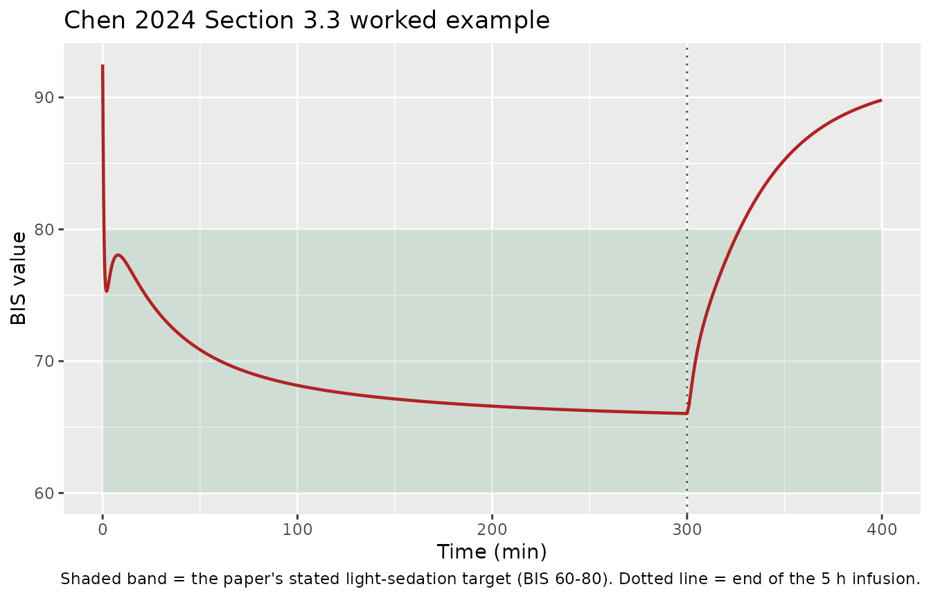
Section 3.3 reports a worked example from the authors’ web dashboard: for a 40-year-old, 60 kg critically ill adult undergoing a 5 h administration with a target BIS of 60-80 (light sedation), the recommended regimen is a 0.1 mg/kg bolus followed by a 0.6 mg/kg/h infusion. This is the single strongest end-to-end check available for this paper, because it exercises the whole chain at once: allometric scaling at the 60 kg reference weight, the parent disposition model, the effect compartment, and every parameter of the sigmoid Imax model.
dash_wt   <- 60
dash_dur  <- 5 * 60                    # 5 h in minutes
dash_rate <- 0.6 * dash_wt / 60        # 0.6 mg/kg/h -> mg/min

dash_times <- sort(unique(c(seq(0, 20, by = 0.25), seq(20, 400, by = 1))))

dash_events <- bind_rows(
  tibble(id = 1L, time = 0, amt = 0.1 * dash_wt,        rate = 0,         evid = 1L, cmt = "central"),
  tibble(id = 1L, time = 0, amt = dash_rate * dash_dur, rate = dash_rate, evid = 1L, cmt = "central"),
  tibble(id = 1L, time = dash_times, amt = NA_real_,    rate = NA_real_,  evid = 0L, cmt = "Cc")
) |>
  mutate(WT = dash_wt) |>
  arrange(time, desc(evid))

dash <- rxode2::rxSolve(
  rxode2::zeroRe(mod), events = dash_events,
  useLinCmt = FALSE, omega = NA, sigma = NA
) |>
  as.data.frame()
#> ℹ parameter labels from comments will be replaced by 'label()'

# The paper's claim has two parts: sedation is reached quickly, and is then
# held at a consistent level. Separate onset from maintenance accordingly.
onset_time <- min(dash$time[dash$BIS <= 80])
maintenance <- dash |> filter(time >= onset_time, time <= dash_dur)

dash_summary <- tibble(
  Quantity = c(
    "BIS at t = 0 (baseline)",
    "Time to first reach the target band, BIS <= 80 (min)",
    "Minimum BIS from onset to end of infusion",
    "Maximum BIS from onset to end of infusion",
    "BIS at end of infusion (t = 300 min)",
    "Remimazolam Cc at end of infusion (ng/mL)",
    "Effect-site concentration at end of infusion (ng/mL)"
  ),
  Value = c(
    round(dash$BIS[dash$time == 0], 1),
    round(onset_time, 2),
    round(min(maintenance$BIS), 1),
    round(max(maintenance$BIS), 1),
    round(dash$BIS[dash$time == dash_dur], 1),
    round(dash$Cc[dash$time == dash_dur], 0),
    round(dash$effect[dash$time == dash_dur], 0)
  )
)

knitr::kable(
  dash_summary,
  caption = paste(
    "Chen 2024 Section 3.3 worked example: 60 kg adult, 0.1 mg/kg bolus +",
    "0.6 mg/kg/h for 5 h. The paper's stated target band is BIS 60-80."
  )
)| Quantity | Value |
|---|---|
| BIS at t = 0 (baseline) | 92.50 |
| Time to first reach the target band, BIS <= 80 (min) | 0.75 |
| Minimum BIS from onset to end of infusion | 66.00 |
| Maximum BIS from onset to end of infusion | 79.40 |
| BIS at end of infusion (t = 300 min) | 66.00 |
| Remimazolam Cc at end of infusion (ng/mL) | 484.00 |
| Effect-site concentration at end of infusion (ng/mL) | 484.00 |
dash |>
  filter(time <= 400) |>
  ggplot(aes(time, BIS)) +
  annotate("rect", xmin = 0, xmax = 400, ymin = 60, ymax = 80,
           alpha = 0.15, fill = "seagreen") +
  geom_vline(xintercept = dash_dur, linetype = "dotted", colour = "grey30") +
  geom_line(linewidth = 0.8, colour = "firebrick") +
  labs(
    x = "Time (min)", y = "BIS value",
    title = "Chen 2024 Section 3.3 worked example",
    caption = paste(
      "Shaded band = the paper's stated light-sedation target (BIS 60-80).",
      "Dotted line = end of the 5 h infusion."
    )
  )
in_band <- with(maintenance, all(BIS >= 60 & BIS <= 80))
fast_onset <- onset_time <= 3
stopifnot(in_band, fast_onset)
cat(sprintf(
  "Onset (BIS <= 80) at %.2f min; BIS held within the paper's 60-80 band from onset to end of infusion: %s\n",
  onset_time, in_band
))
#> Onset (BIS <= 80) at 0.75 min; BIS held within the paper's 60-80 band from onset to end of infusion: TRUE
The packaged model reproduces both halves of the paper’s claim: sedation is reached within the paper’s stated 3 min, and BIS is then held inside the stated 60-80 light-sedation band for the rest of the 5 h administration. A hand calculation agrees with the plateau: at the infusion rate of 0.6 mg/min the steady-state concentration is 0.6 / 1.21 = 0.496 mg/L = 496 ng/mL, within 2 percent of the published IC50 of 504 ng/mL, so the effect is close to half of Imax and BIS settles near 92.5 - 54.5/2 = 65.3.
This is the strongest available end-to-end check on the extraction.
It is sensitive to the reference weight of Equation (5), to remimazolam
CL and V1, to ke0, and to all four parameters of the
sigmoid Imax model simultaneously; it also discriminates the corrected
Equation (8) denominator from the printed one (under the printed
multiplicative form the effect term is independent of concentration and
no dose would move BIS at all).
Assumptions and deviations
Equation (8) is printed with a multiplication where a sum belongs
Chen 2024 prints the sigmoid Imax model as
BIS = BIS_baseline - (Imax * CE^Hill) / (IC50^Hill * CE^Hill)with a multiplication in the denominator. As
printed, CE^Hill cancels and the whole effect term
collapses to the constant Imax / IC50^Hill, which is
independent of concentration – the equation would describe a fixed BIS
offset present even at zero drug, and no sigmoid at all. It also
contradicts the paper’s own definition of IC50 immediately
below the equation as “the concentration at half-maximum effect”, which
holds only for the summed form. The model file therefore encodes the
standard sigmoid Imax denominator,
BIS = BIS_baseline - (Imax * CE^Hill) / (IC50^Hill + CE^Hill)This reading is confirmed numerically by the Section 3.3 worked example reproduced above, which lands inside the paper’s stated target band only under the summed form.
Note also that Equation (8) is subtractive
(BIS_baseline - ...), not multiplicative, so
Imax = 54.5 is in absolute BIS units rather than a
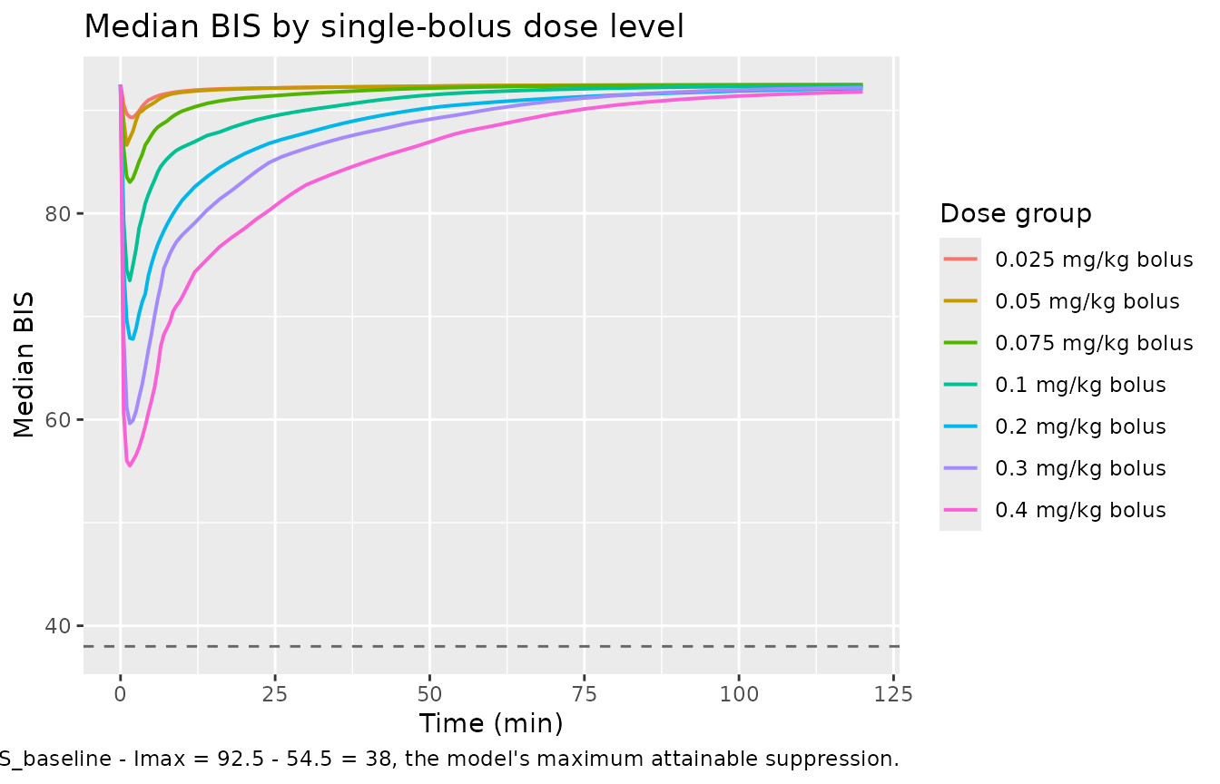
fraction; maximum attainable suppression is
92.5 - 54.5 = 38 BIS units.
Inter-individual variability reported as percentages
Tables 3 and 4 report BSV as percentages for an exponential BSV model
(Equation 1) without stating whether the percentage is a coefficient of
variation or omega * 100. They are read here as
coefficients of variation and converted with
omega^2 = log(CV^2 + 1), which is the package’s convention
for exponential IIV reported as a percentage. The choice is immaterial
for the small IIVs and shifts omega by at most about 6
percent for the largest (V1, 55 percent).
Text-versus-table conflicts, resolved in favour of the tables
Several statements in the running text disagree with the final parameter tables. In each case the table value is used, because the tables carry RSEs and shrinkage values and are labelled as the final model estimates.
- Section 3.2.1 states that BSV was placed on “CL, central volume (V1), peripheral volume (V3), and intercompartmental clearance (Q3)”. Table 3 instead reports IIV on CL, V1, Q2, V2, and Ktr, and reports none on Q3 or V3. The model follows Table 3.
- Section 3.2.2 states that BSV was incorporated into “Imax and IC50”. Table 4 Cont. instead reports IIV on Imax and Hill, and none on IC50. The model follows Table 4.
- Section 3.2.1 gives remimazolam CL as “1.36” L/min in the sentence comparing it with CNS 7054, while Table 3 reports 1.21 L/min. The Discussion’s “1.2 L/min/60 kg” agrees with Table 3, as does the 60 kg reference weight of Equation (5), so 1.21 is used.
- The Discussion quotes
Imaxas 54.1 andke0as 1.09 1/min, against Table 4’s 54.5 and 1.38 1/min. The table values are used. - The Discussion quotes the BSV of the central volume as 56.8 percent against Table 3’s 55 percent. The table value is used.
Metabolite stoichiometry
Chen 2024 states that “all remimazolam was converted into CNS 7054 in a first-order process” but gives no molar or mass conversion factor. The model therefore transfers amount 1:1, so the fitted CNS 7054 volumes and clearance are apparent values expressed in remimazolam-mass equivalents. The two molecular weights differ by only about 3 percent (parent 439, metabolite 425.1, read from the LC/MS/MS precursor ions reported in Section 2.1.3), which is within the 3-5 percent RSEs of the metabolite disposition parameters, so the distinction is not resolvable from the published data.
Residual-error correlation between analytes is not encodable
Table 3 reports COR (remimazolam _CNS7054) = 0.0066 for
the correlation of residual errors between the two analytes, which were
measured in the same samples. nlmixr2’s error model is specified per
endpoint and cannot express a correlation between the residuals of two
endpoints, so this term is omitted. The reported figure is also
ambiguous: read as a correlation coefficient it is essentially zero
(which would contradict the text’s claim that a correlation “was
identified”), whereas read as a $SIGMA block covariance it
implies a correlation of about 0.44 against the two reported
proportional error variances. Neither reading changes the typical-value
predictions.
Scope of the allometric scaling
Equation (5) applies allometry to “the PK models”, with exponents of
0.75 for clearance and 1 for volume. It is applied here to every
clearance term (CLp, Q2, Q3, CLm, Q4) and every volume term (V1, V2, V3,
V5, V6) of both the remimazolam and the CNS 7054 disposition models. The
transit rate constant Ktr and the effect-compartment rate
constant ke0 are left unscaled: neither is a clearance or a
volume, and the paper does not state an exponent for a first-order rate
constant.
Figure axis labels and one concentration figure in the text are inconsistent
Two reporting defects in the source do not affect any encoded parameter but are worth recording:
- The y-axis of Figure 3 panels A and B is labelled “Concentration (mol/L)” while carrying values from about 1 to 30,000; the analyte concentrations are in ng/mL throughout the rest of the paper.
- Section 3.2.1 describes 43.13 ng/mL as “minimal compared to the concentrations of remimazolam, reaching a high of 30,000 ng/mL”. The 30,000 figure matches the axis range of the CNS 7054 goodness-of-fit panel (Figure 2B), not remimazolam, and exceeds the paper’s own stated 2-2000 ng/mL assay calibration range. The packaged model predicts a remimazolam Cmax of 1500 ng/mL at the highest bolus dose (0.4 mg/kg at 62.5 kg), which sits inside the calibration range.
Simulation assumptions
- Body weights are drawn from a normal distribution (mean 62.5 kg, SD 5.5 kg) truncated to the published 52-75 kg range; the paper reports only the median and range, not the distributional shape.
- Age, height, and sex are not simulated because no covariate on any of them was retained in either the PK or the PD model.
- All parameter values come from the paper’s Tables 3 and 4 and Equation (5). No value was taken from author correspondence, figure digitisation, or an upstream model.