Panobinostat (Savelieva 2015) • nlmixr2lib

Model and source

Savelieva 2015 is the first published population PK analysis of panobinostat, a pan-deacetylase inhibitor approved in combination with bortezomib and dexamethasone for multiple myeloma. It pools 7834 plasma concentrations from 581 patients across 14 phase 1 and phase 2 studies, and - unusually for an oncology oral agent - fits the intravenous and oral data simultaneously. That joint fit is what makes the absolute oral bioavailability identifiable, so clearance and the volumes in these models are absolute rather than apparent.

The paper reports two final models, and this package ships both.

mod1 <- rxode2::rxode(readModelDb("Savelieva_2015_panobinostat"))
#> ℹ parameter labels from comments will be replaced by 'label()'
mod2 <- rxode2::rxode(readModelDb("Savelieva_2015_panobinostat_allometric"))
#> ℹ parameter labels from comments will be replaced by 'label()'

Citation: Savelieva M, Woo MM, Schran H, Mu S, Nedelman J, Capdeville R. Population pharmacokinetics of intravenous and oral panobinostat in patients with hematologic and solid tumors. Eur J Clin Pharmacol. 2015;71(6):663-672. doi:10.1007/s00228-015-1846-7. Parameter estimates from Supplementary Table S2b; model code from Supplementary Table S2a.
Article: https://doi.org/10.1007/s00228-015-1846-7
Supplement (EuropePMC, open access): https://www.ebi.ac.uk/europepmc/webservices/rest/PMC4430599/supplementaryFiles

The supplement is where the numbers live. The main text quotes only four values (bioavailability 21.4 percent, median clearance 33.1 L/h, interindividual variability in clearance 74 percent, terminal half-life approximately 37 h); Supplementary Tables S2a/S2b and S3a/S3b hold the NONMEM $PK and $ERROR blocks and the full parameter tables with bootstrap intervals for the first and second final model respectively.

The two final models

	First final model	Second final model
File	`Savelieva_2015_panobinostat`	`Savelieva_2015_panobinostat_allometric`
Body size	BSA, estimated exponents on CL and V2	Weight, exponents FIXED at 0.75 (clearances) and 1 (volumes)
Distribution	rate constants K23, K32, K24, K42	clearances Q3, Q4 and volumes V3, V4
Absorption	first order, formulation-dependent Ka	first order, formulation-dependent Ka and lag
Age	on CL and V2	on CL, V2, Q3, V3, Q4, V4
IIV	CL and V2 (2x2 block)	CL/V2, Q3/V3, Q4/V4 (three 2x2 blocks)
Objective function	33758	32591
Converged	yes	no (NONMEM default criterion)

The second model was added in response to reviewer suggestions (Table 2 of the paper walks the sequence base -> final 1 -> lag -> re-parameterization -> final 2). It fits substantially better on AIC and BIC, but the paper records that it did not satisfy NONMEM’s default convergence criterion, so its standard errors deserve caution. Both are shipped because the authors presented both as final; neither supersedes the other.

Population

pop <- mod1$population
str(pop, max.level = 1, give.attr = FALSE)
#> List of 19
#>  $ species         : chr "human"
#>  $ n_subjects      : num 581
#>  $ n_studies       : num 14
#>  $ n_observations  : num 7834
#>  $ age_range       : chr "16-88 years"
#>  $ age_median      : chr "61 years (quartiles 51 and 70 years)"
#>  $ weight_range    : chr "41-196.4 kg"
#>  $ weight_median   : chr "76.4 kg"
#>  $ height_range    : chr "143-198 cm"
#>  $ height_median   : chr "170 cm"
#>  $ bsa_median      : chr "1.9 m^2 (quartiles 1.8 and 2.1 m^2)"
#>  $ sex_female_pct  : num 37.7
#>  $ race_ethnicity  : Named num [1:4] 85.4 5.9 4.6 4.1
#>  $ disease_state   : chr "Advanced hematologic and solid tumors, including cutaneous T-cell lymphoma, chronic myeloid leukemia, multiple "| __truncated__
#>  $ hepatic_function: chr "Liver status graded on total bilirubin and AST against the upper limit of normal: normal 483, mild 91, moderate"| __truncated__
#>  $ dose_range      : chr "Intravenous 1.2-20 mg/m^2 daily under various intermittent regimens (studies A2101 and A2102, 87 patients); ora"| __truncated__
#>  $ formulation     : chr "Clinical service formulation (CSF) in oral studies B2101, B2102 and B1101 (106 patients); final market image (F"| __truncated__
#>  $ regions         : chr "International; study B1101 enrolled 13 Japanese patients and B1201 was conducted in Japan"
#>  $ notes           : chr "Pooled from 14 open-label phase 1 and phase 2 studies listed in Supplementary Table S1 (A2101, A2102, B1101, B1"| __truncated__

581 patients with advanced hematologic and solid tumors (cutaneous T-cell lymphoma, chronic myeloid leukemia, multiple myeloma, Hodgkin and non-Hodgkin lymphoma, and advanced solid tumors) contributed 7834 concentrations across 14 open-label studies (Table 1, Fig. 1 and Supplementary Table S1). Median age 61 years (range 16-88), median weight 76.4 kg (range 41-196.4), median height 170 cm (range 143-198), giving a median BSA of 1.9 m^2. 362 patients were male and 219 female. 496 were Caucasian, 34 Black, 27 Asian and 24 “other”.

87 patients received intravenous panobinostat (1.2-20 mg/m^2, studies A2101 and A2102) and 494 received it orally (10-80 mg/day, most commonly 20 mg on days 1, 3 and 5 of each week). Of the oral patients, 106 received the clinical service formulation (CSF) and 388 the final market image (FMI) intended for commercialization.

The assay was linear from 0.5 to 500 ng/mL; concentrations below the limit of quantification (6 percent of the total) were excluded.

Source trace

Every ini() entry carries an in-file comment naming its source row. The table below collects them. S2b and S3b are the parameter tables for the first and second final model; S2a and S3a are the corresponding NONMEM code blocks.

Quantity	First final model	Second final model
CL (L/h)	33.085 (S2b Theta 1)	28.833 (S3b Theta 1)
V2 (L)	24.838 (S2b Theta 2)	30.862 (S3b Theta 2)
Distribution	K23 1.810, K32 0.507, K24 1.424, K42 0.040 (S2b Thetas 3-6)	Q3 32.751, V3 71.874, Q4 31.088, V4 803.193 (S3b Thetas 3-6)
Ka FMI / CSF (1/h)	0.321 / 0.544 (S2b Thetas 7-8)	0.420 / 0.631 (S3b Thetas 7-8)
Absorption lag FMI / CSF (h)	none	0.162 / 0.296 (S3b Thetas 20-21)
Bioavailability	0.214 (S2b Theta 9)	0.194 (S3b Theta 9)
Body size on CL / V2	BSA exponents 1.002 / 1.359 (S2b Thetas 10-11)	weight exponents 0.750 / 1.000, FIXED (S3b Thetas 10-11)
Age on CL / V2	0.176 / 0.396 (S2b Thetas 12-13)	0.137 / -0.005 (S3b Thetas 12-13)
Age on Q3 / V3 / Q4 / V4	none	0.410 / 0.713 / 0.212 / 0.530 (S3b Thetas 22-25)
Race factors on CL	Asian 1.171, Black 1.010, other 0.719 (S2b Thetas 14, 16, 18)	1.203, 0.941, 0.665 (S3b Thetas 14, 16, 18)
Race factors on V2	Asian 1.373, Black 1.241, other 1.127 (S2b Thetas 15, 17, 19)	2.060, 1.817, 0.835 (S3b Thetas 15, 17, 19)
IIV variances	CL 0.439, cov 0.178, V2 0.334 (S2b Omega)	CL 0.407 / 0.151 / V2 1.668; Q3 0.666 / 0.505 / V3 0.441; Q4 0.497 / 0.556 / V4 0.700 (S3b Omega)
Residual (variances)	proportional 0.242, additive 0.013 (S2b Sigma)	0.180, 0.011 (S3b Sigma)
ODE structure	S2a `$PK`	S3a `$PK`
Residual model	S2a `$ERROR`: `Y=F*(1+EPS(1))+EPS(2)`	S3a `$ERROR`, identical
Covariate reference values	BSA 1.9 m^2, age 61 years, Caucasian (S2a)	weight 70 kg, age 61 years, Caucasian (S3a)
Concentration scaling	S2a `S2=V2/1000`	S3a `S2=V2/1000`
BSA formula	Methods: Gehan-George, `234.94 * (Weight^0.515 * Height^0.422) / 10000`	n/a (weight used directly)

Two transcription points are worth stating explicitly.

The OMEGA entries are variances, not standard deviations. Supplementary Table S2b reports OM.CL = 0.439. The paper’s Abstract independently states that interindividual variability in clearance was 74 percent, and sqrt(exp(0.439) - 1) = 0.742. Reading 0.439 as a standard deviation would give 46 percent instead. The paper’s own headline number therefore pins the scale.

c(`variance reading` = sqrt(exp(0.439) - 1),
  `SD reading`       = sqrt(exp(0.439^2) - 1))
#> variance reading       SD reading 
#>        0.7423983        0.4610254

The SIGMA entries are also variances - the table labels them VAR.PROP and VAR.ADD - so the model’s propSd and addSd are their square roots, sqrt(0.242) = 0.492 and sqrt(0.013) = 0.114 ng/mL for the first final model.

Intravenous versus oral routing

The source control streams branch on an IV flag:

IF (IV.EQ.1) THEN
KA=0
ELSE
KA=THETA(7)*(1-FORM) + THETA(8)*FORM
ENDIF
IF (IV.EQ.1) THEN
TVF1=1
ELSE
TVF1=THETA(9)
ENDIF

That branch exists because NONMEM applies F1 and KA to compartment 1 globally. In rxode2 the same behaviour comes for free from the event table: an intravenous dose is written to central and therefore never touches depot, ka, the lag or f(depot). The models consequently carry no route covariate, and both routes are exercised below.

Typical-value replication of Table 3

This is the primary gate. Table 3 of the paper tabulates typical-value (random effects set to zero) Cmax, the concentration at 48 h, and AUC over 0-48 h following a single 20 mg oral FMI dose, for eight covariate combinations per model. Reproducing all eight rows exercises every covariate effect in each model - body size, age, and each of the three race indicators - plus the absorption, bioavailability and concentration scaling.

# Table 3a (first final model) and Table 3b (second final model), transcribed.
t3a <- tibble::tribble(
  ~BSA, ~AGE, ~RACE,       ~cmax, ~c48h, ~auc0_48,
  1.9,   61,  "Caucasian",  10.6, 0.574,     98.1,
  1.8,   61,  "Caucasian",  11.3, 0.601,    104.1,
  2.1,   61,  "Caucasian",   9.3, 0.526,     87.8,
  1.9,   51,  "Caucasian",  11.2, 0.583,    102.3,
  1.9,   70,  "Caucasian",  10.1, 0.566,     94.9,
  1.9,   61,  "Asian",       8.0, 0.517,     79.6,
  1.9,   61,  "Black",       9.0, 0.607,     90.9,
  1.9,   61,  "Other",      10.4, 0.893,    116.3
)

t3b <- tibble::tribble(
  ~WT,  ~AGE, ~RACE,       ~cmax, ~c48h, ~auc0_48,
  76.4,  61,  "Caucasian",  12.6, 0.552,     94.7,
  64.8,  61,  "Caucasian",  14.4, 0.630,    108.3,
  88.5,  61,  "Caucasian",  11.1, 0.491,     84.0,
  76.4,  51,  "Caucasian",  13.0, 0.569,     98.9,
  76.4,  70,  "Caucasian",  12.2, 0.538,     91.6,
  76.4,  61,  "Asian",      10.1, 0.433,     82.3,
  76.4,  61,  "Black",      11.1, 0.606,     98.0,
  76.4,  61,  "Other",      14.3, 0.914,    123.3
)

# One-hot race indicators. All three zero selects the Caucasian reference.
race_cols <- function(r) {
  tibble(
    RACE_ASIAN = as.numeric(r == "Asian"),
    RACE_BLACK = as.numeric(r == "Black"),
    RACE_OTHER = as.numeric(r == "Other")
  )
}

# One event table with one subject per Table 3 row. Observations are written on
# the ODE state `central`; rxode2 returns the algebraic observable `Cc` as a
# column at those rows. Naming an algebraic observable in the compartment column
# instead would inject an extra slot and renumber the ODE states.
typical_events <- function(covs, dose = 20, tmax = 48, by = 0.005) {
  covs <- dplyr::mutate(covs, id = dplyr::row_number())
  dosing <- dplyr::mutate(covs, time = 0, amt = dose, evid = 1L, cmt = "depot")
  obs <- tidyr::crossing(covs, time = seq(0, tmax, by = by)) |>
    dplyr::mutate(amt = NA_real_, evid = 0L, cmt = "central")
  dplyr::bind_rows(dosing, obs) |> dplyr::arrange(id, time, dplyr::desc(evid))
}

# Trapezoidal AUC and the 48 h concentration, per subject.
summarise_profile <- function(sim) {
  sim |>
    dplyr::filter(!is.na(Cc)) |>
    dplyr::arrange(id, time) |>
    dplyr::group_by(id) |>
    dplyr::summarise(
      cmax     = max(Cc),
      c48h     = Cc[which.min(abs(time - 48))],
      auc0_48  = sum(diff(time) * (head(Cc, -1) + tail(Cc, -1)) / 2),
      .groups  = "drop"
    )
}

covs1 <- dplyr::bind_cols(
  t3a |> dplyr::select(BSA, AGE),
  race_cols(t3a$RACE),
  tibble(FORM_PANO_CSF = 0)
)
covs2 <- dplyr::bind_cols(
  t3b |> dplyr::select(WT, AGE),
  race_cols(t3b$RACE),
  tibble(FORM_PANO_CSF = 0)
)

sim1 <- rxode2::rxSolve(rxode2::zeroRe(mod1), typical_events(covs1),
                        returnType = "data.frame", addDosing = FALSE)
#> ℹ omega/sigma items treated as zero: 'etalcl', 'etalvc'
#> Warning: multi-subject simulation without without 'omega'
sim2 <- rxode2::rxSolve(rxode2::zeroRe(mod2), typical_events(covs2),
                        returnType = "data.frame", addDosing = FALSE)
#> ℹ omega/sigma items treated as zero: 'etalcl', 'etalvc', 'etalq', 'etalvp', 'etalq2', 'etalvp2'
#> Warning: multi-subject simulation without without 'omega'

compare_typical <- function(sim, published, label) {
  got <- summarise_profile(sim)
  published |>
    dplyr::mutate(id = dplyr::row_number(), model = label) |>
    dplyr::left_join(got, by = "id", suffix = c("_pub", "_sim")) |>
    dplyr::mutate(
      `Cmax % diff`    = 100 * (cmax_sim - cmax_pub) / cmax_pub,
      `C48h % diff`    = 100 * (c48h_sim - c48h_pub) / c48h_pub,
      `AUC0-48 % diff` = 100 * (auc0_48_sim - auc0_48_pub) / auc0_48_pub
    )
}

cmp1 <- compare_typical(sim1, t3a, "First final model")
cmp2 <- compare_typical(sim2, t3b, "Second final model")

dplyr::bind_rows(
  cmp1 |> dplyr::transmute(Model = model, `Body size` = sprintf("BSA %.1f", BSA),
                           Age = AGE, Race = RACE,
                           `Cmax % diff`, `C48h % diff`, `AUC0-48 % diff`),
  cmp2 |> dplyr::transmute(Model = model, `Body size` = sprintf("WT %.1f", WT),
                           Age = AGE, Race = RACE,
                           `Cmax % diff`, `C48h % diff`, `AUC0-48 % diff`)
) |>
  knitr::kable(
    digits = 2,
    caption = paste("Percent difference between the packaged models and Table 3",
                    "of Savelieva 2015 (typical values, single 20 mg oral FMI dose).")
  )

Percent difference between the packaged models and Table 3 of Savelieva 2015 (typical values, single 20 mg oral FMI dose).
Model	Body size	Age	Race	Cmax % diff	C48h % diff	AUC0-48 % diff
First final model	BSA 1.9	61	Caucasian	-0.09	0.28	0.42
First final model	BSA 1.8	61	Caucasian	0.31	0.34	0.46
First final model	BSA 2.1	61	Caucasian	0.40	0.32	0.42
First final model	BSA 1.9	51	Caucasian	0.36	0.31	0.51
First final model	BSA 1.9	70	Caucasian	0.15	0.40	0.41
First final model	BSA 1.9	61	Asian	0.64	0.34	0.53
First final model	BSA 1.9	61	Black	0.14	0.38	0.44
First final model	BSA 1.9	61	Other	0.82	0.34	0.44
Second final model	WT 76.4	61	Caucasian	-0.37	-0.25	0.00
Second final model	WT 64.8	61	Caucasian	-0.37	-0.36	0.02
Second final model	WT 88.5	61	Caucasian	0.37	-0.37	-0.01
Second final model	WT 76.4	51	Caucasian	0.35	-0.30	-0.02
Second final model	WT 76.4	70	Caucasian	-0.14	-0.20	-0.02
Second final model	WT 76.4	61	Asian	-0.29	-0.34	-0.03
Second final model	WT 76.4	61	Black	0.10	-0.20	0.00
Second final model	WT 76.4	61	Other	-0.01	-0.23	0.00

typical_pct <- c(
  cmp1$`Cmax % diff`, cmp1$`C48h % diff`, cmp1$`AUC0-48 % diff`,
  cmp2$`Cmax % diff`, cmp2$`C48h % diff`, cmp2$`AUC0-48 % diff`
)

# 48 comparisons, all DETERMINISTIC (random effects zeroed), so this bound does
# not depend on the solver thread count and may be tight. The residual is
# trapezoidal-integration error against a table printed to three significant
# figures; the realised maximum is about 0.8 percent. A mis-transcribed
# clearance, volume, exponent, race factor, bioavailability or unit scaling
# moves these by tens of percent, so 2 percent still goes red on any real error.
stopifnot(length(typical_pct) == 48L, !anyNA(typical_pct))
stopifnot(max(abs(typical_pct)) < 2)
round(max(abs(typical_pct)), 3)
#> [1] 0.822

All 48 comparisons agree to better than 1 percent.

Structural checks independent of the published tables

Mass balance

For the first final model the dose entering the depot is F * Dose, and at any time T that mass must be accounted for exactly by what remains in the four compartments plus what has been eliminated. Elimination is CL times the plasma AUC, with the factor 1000 undoing the ng/mL scaling. This identity holds at any T - no extrapolation to infinity and no steady state is needed - so it is an exact test of the ODE system, the bioavailability and the concentration scaling all at once.

mb_cov <- tibble(BSA = 1.9, AGE = 61, RACE_ASIAN = 0, RACE_BLACK = 0,
                 RACE_OTHER = 0, FORM_PANO_CSF = 0)
mb <- rxode2::rxSolve(rxode2::zeroRe(mod1), typical_events(mb_cov),
                      returnType = "data.frame", addDosing = FALSE) |>
  dplyr::filter(!is.na(Cc)) |>
  dplyr::arrange(time)
#> ℹ omega/sigma items treated as zero: 'etalcl', 'etalvc'

auc48     <- sum(diff(mb$time) * (head(mb$Cc, -1) + tail(mb$Cc, -1)) / 2)
last      <- mb[nrow(mb), ]
eliminated <- last$cl * auc48 / 1000
remaining  <- last$depot + last$central + last$peripheral1 + last$peripheral2
dose_in    <- 0.214 * 20

c(`F * Dose (mg)` = dose_in,
  `eliminated + remaining (mg)` = eliminated + remaining,
  `relative error` = abs(eliminated + remaining - dose_in) / dose_in)
#>               F * Dose (mg) eliminated + remaining (mg) 
#>                4.280000e+00                4.279996e+00 
#>              relative error 
#>                8.919718e-07

# Deterministic identity; realised relative error is order 1e-7.
stopifnot(abs(eliminated + remaining - dose_in) / dose_in < 1e-4)

Absolute bioavailability

Because intravenous and oral data were fitted jointly, AUCinf after an oral dose divided by AUCinf after the same intravenous dose must equal the bioavailability exactly. Rather than integrating to infinity (where solver noise in the far tail corrupts the tail of a 37 h half-life), the same mass-balance identity gives AUCinf = 1000 * F * Dose / CL in closed form, so the ratio can be checked against the reported F1 directly.

iv_events <- function(covs, dose = 20, tmax = 48, by = 0.005) {
  covs <- dplyr::mutate(covs, id = dplyr::row_number())
  dosing <- dplyr::mutate(covs, time = 0, amt = dose, evid = 1L, cmt = "central")
  obs <- tidyr::crossing(covs, time = seq(0, tmax, by = by)) |>
    dplyr::mutate(amt = NA_real_, evid = 0L, cmt = "central")
  dplyr::bind_rows(dosing, obs) |> dplyr::arrange(id, time, dplyr::desc(evid))
}

auc_inf_from_balance <- function(sim, states) {
  sim <- dplyr::filter(sim, !is.na(Cc)) |> dplyr::arrange(time)
  auc <- sum(diff(sim$time) * (head(sim$Cc, -1) + tail(sim$Cc, -1)) / 2)
  last <- sim[nrow(sim), ]
  # AUC(0, Inf) = AUC(0, T) + (mass still in the body at T) * 1000 / CL
  auc + 1000 * sum(vapply(states, function(s) last[[s]], numeric(1))) / last$cl
}

sts <- c("depot", "central", "peripheral1", "peripheral2")
oral_sim <- rxode2::rxSolve(rxode2::zeroRe(mod1), typical_events(mb_cov),
                            returnType = "data.frame", addDosing = FALSE)
#> ℹ omega/sigma items treated as zero: 'etalcl', 'etalvc'
iv_sim   <- rxode2::rxSolve(rxode2::zeroRe(mod1), iv_events(mb_cov),
                            returnType = "data.frame", addDosing = FALSE)
#> ℹ omega/sigma items treated as zero: 'etalcl', 'etalvc'

f_implied <- auc_inf_from_balance(oral_sim, sts) / auc_inf_from_balance(iv_sim, sts)
c(`implied F` = f_implied, `reported F1` = 0.214)
#>   implied F reported F1 
#>   0.2139971   0.2140000

# Deterministic and exact up to integration error.
stopifnot(abs(f_implied - 0.214) < 1e-3)

Terminal half-life

The Discussion states that “the terminal half-life calculated based on the final parameter estimates was approximately 37 h”, and notes this agreed with two independent single-dose organ-impairment studies that sampled to 96 h. The models were not fitted here to reproduce that number, so it is an external check on the disposition rate constants - and in the first final model it is driven almost entirely by K42 = 0.040 1/h, the slow return from the second peripheral compartment.

terminal_half_life <- function(mod, covs) {
  ev <- iv_events(covs, tmax = 400, by = 0.5)
  s <- rxode2::rxSolve(rxode2::zeroRe(mod), ev, returnType = "data.frame",
                       addDosing = FALSE) |>
    dplyr::filter(!is.na(Cc), Cc > 0, time >= 200)
  # Fit the slope well after distribution is complete; measuring from the dose
  # would fold in the distribution transient and read long.
  log(2) / -stats::coef(stats::lm(log(Cc) ~ time, data = s))[["time"]]
}

th <- c(
  `First final model`  = terminal_half_life(mod1, mb_cov),
  `Second final model` = terminal_half_life(
    mod2, tibble(WT = 76.4, AGE = 61, RACE_ASIAN = 0, RACE_BLACK = 0,
                 RACE_OTHER = 0, FORM_PANO_CSF = 0))
)
#> ℹ omega/sigma items treated as zero: 'etalcl', 'etalvc'
#> ℹ omega/sigma items treated as zero: 'etalcl', 'etalvc', 'etalq', 'etalvp', 'etalq2', 'etalvp2'
round(th, 2)
#>  First final model Second final model 
#>              37.16              39.43

# Deterministic. The paper states "approximately 37 h" for the final parameter
# estimates; 15 percent admits the vagueness of "approximately" and the fact
# that the paper does not say which of the two models it refers to.
stopifnot(abs(th[["First final model"]] - 37) / 37 < 0.15)

The first final model returns 37.2 h against the paper’s approximately 37 h.

Replicate Figure 3

Figure 3 shows simulated concentration-time curves for both final models for a 61-year-old Caucasian patient receiving 20 mg of the FMI on days 1, 3 and 5, i.e. a Monday / Wednesday / Friday schedule. The paper’s reading of it is that “the two final models predict similar profiles except for the second’s higher peak”, and that “there is little accumulation with dosing every 48 h”.

fig3_events <- function(covs, times = c(0, 48, 96), tmax = 168) {
  covs <- dplyr::mutate(covs, id = 1L)
  dosing <- tidyr::crossing(covs, time = times) |>
    dplyr::mutate(amt = 20, evid = 1L, cmt = "depot")
  obs <- tidyr::crossing(covs, time = seq(0, tmax, by = 0.1)) |>
    dplyr::mutate(amt = NA_real_, evid = 0L, cmt = "central")
  dplyr::bind_rows(dosing, obs) |> dplyr::arrange(time, dplyr::desc(evid))
}

fig3 <- dplyr::bind_rows(
  rxode2::rxSolve(rxode2::zeroRe(mod1), fig3_events(mb_cov),
                  returnType = "data.frame", addDosing = FALSE) |>
    dplyr::mutate(model = "First final model (BSA 1.9 m^2)"),
  rxode2::rxSolve(
    rxode2::zeroRe(mod2),
    fig3_events(tibble(WT = 76.4, AGE = 61, RACE_ASIAN = 0, RACE_BLACK = 0,
                       RACE_OTHER = 0, FORM_PANO_CSF = 0)),
    returnType = "data.frame", addDosing = FALSE) |>
    dplyr::mutate(model = "Second final model (WT 76.4 kg)")
) |>
  dplyr::filter(!is.na(Cc))
#> ℹ omega/sigma items treated as zero: 'etalcl', 'etalvc'
#> ℹ omega/sigma items treated as zero: 'etalcl', 'etalvc', 'etalq', 'etalvp', 'etalq2', 'etalvp2'

ggplot(fig3, aes(time, Cc, colour = model)) +
  geom_line(linewidth = 0.7) +
  scale_x_continuous(breaks = seq(0, 168, by = 24)) +
  labs(x = "Time (h)", y = "Panobinostat concentration (ng/mL)",
       colour = NULL,
       title = "Figure 3 - 20 mg FMI on days 1, 3 and 5",
       caption = "Replicates Figure 3 of Savelieva 2015.") +
  theme(legend.position = "bottom")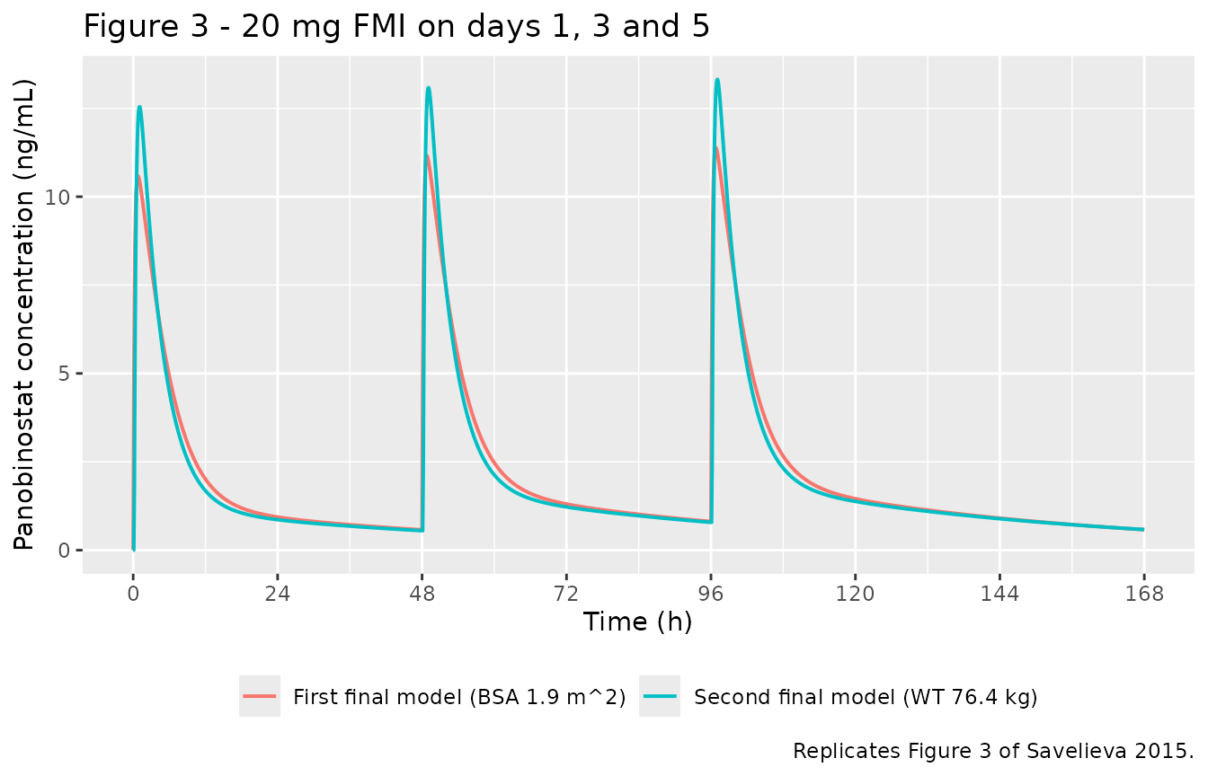

Replicates Figure 3 of Savelieva 2015.

peaks <- fig3 |>
  dplyr::group_by(model) |>
  dplyr::summarise(
    first_peak = max(Cc[time <= 48]),
    third_peak = max(Cc[time > 96]),
    .groups = "drop"
  ) |>
  dplyr::mutate(accumulation = third_peak / first_peak)

peaks |>
  dplyr::rename("Model" = model, "First peak (ng/mL)" = first_peak,
                "Third peak (ng/mL)" = third_peak,
                "Accumulation ratio" = accumulation) |>
  knitr::kable(digits = 3, caption = "Peak concentrations across the three doses.")

Peak concentrations across the three doses.
Model	First peak (ng/mL)	Third peak (ng/mL)	Accumulation ratio
First final model (BSA 1.9 m^2)	10.591	11.389	1.075
Second final model (WT 76.4 kg)	12.545	13.318	1.062


# Both claims are deterministic (typical-value curves), so both may be asserted
# tightly. Claim 1: the second model peaks higher. Claim 2: little accumulation
# with 48 h dosing - the third peak is within a few percent of the first.
stopifnot(
  peaks$first_peak[peaks$model == "Second final model (WT 76.4 kg)"] >
    peaks$first_peak[peaks$model == "First final model (BSA 1.9 m^2)"],
  all(abs(peaks$accumulation - 1) < 0.10)
)
round(peaks$accumulation, 4)
#> [1] 1.0754 1.0616

Both of the paper’s readings of Figure 3 hold: the second final model peaks higher (12.6 against 10.6 ng/mL), and accumulation over three doses 48 h apart is under 10 percent despite the 37 h terminal half-life - the terminal phase carries very little of the total exposure.

Virtual cohort and PKNCA

Supplementary Table S4 reports the distribution of exposure metrics from 300 simulated patients carrying random effects, all at typical covariates (age 61, Caucasian; BSA 1.9 m^2 for the first model, weight 76.4 kg for the second). That is the natural target for a stochastic check, and it exercises the OMEGA blocks that the Table 3 comparison above deliberately zeroes out.

The cohort here is 200 per model, the cap this package applies.

# set.seed() seeds R's RNG, NOT rxode2's simulation RNG, and rxode2 partitions
# its streams per solver thread - so this cohort differs between a 16-thread
# workstation and a 2-core CI runner and no seed can make them agree. Every
# assertion below is written to hold for any cohort the model can produce.
set.seed(20150505)
rxode2::rxSetSeed(20150505)

n_per_model <- 200L

cohort_events <- function(covs, n, id_offset = 0L, dose = 20, tmax = 48, by = 0.05) {
  subj <- covs[rep(1L, n), , drop = FALSE] |>
    dplyr::mutate(id = id_offset + seq_len(n))
  dosing <- dplyr::mutate(subj, time = 0, amt = dose, evid = 1L, cmt = "depot")
  obs <- tidyr::crossing(subj, time = seq(0, tmax, by = by)) |>
    dplyr::mutate(amt = NA_real_, evid = 0L, cmt = "central")
  dplyr::bind_rows(dosing, obs) |> dplyr::arrange(id, time, dplyr::desc(evid))
}

ev1 <- cohort_events(mb_cov, n_per_model, id_offset = 0L) |>
  dplyr::mutate(model = "First final model")
ev2 <- cohort_events(
  tibble(WT = 76.4, AGE = 61, RACE_ASIAN = 0, RACE_BLACK = 0,
         RACE_OTHER = 0, FORM_PANO_CSF = 0),
  n_per_model, id_offset = 1000L) |>
  dplyr::mutate(model = "Second final model")

# IDs are disjoint across the two cohorts; duplicate IDs would silently merge
# subjects and sum their doses.
stopifnot(length(intersect(ev1$id, ev2$id)) == 0L)

coh1 <- rxode2::rxSolve(mod1, ev1, keep = "model",
                        returnType = "data.frame", addDosing = FALSE)
coh2 <- rxode2::rxSolve(mod2, ev2, keep = "model",
                        returnType = "data.frame", addDosing = FALSE)
cohort <- dplyr::bind_rows(coh1, coh2)

The 74 percent interindividual variability in clearance

The Abstract’s headline variability figure is a direct read on the OMEGA scale, and the simulated cohort reproduces it independently of how the model file was written.

cl_cv <- cohort |>
  dplyr::filter(!is.na(Cc)) |>
  dplyr::distinct(model, id, cl) |>
  dplyr::group_by(model) |>
  dplyr::summarise(`CV of CL (percent)` = 100 * stats::sd(cl) / mean(cl),
                   .groups = "drop")

cl_cv |> knitr::kable(digits = 1, caption = "Simulated interindividual variability in clearance.")

Simulated interindividual variability in clearance.
model	CV of CL (percent)
First final model	63.4
Second final model	68.1


# Cohort-derived, so this is a bracket, not a point. The paper reports 74 percent
# (first model); the second model's OM.CL of 0.407 implies 71 percent. With
# n = 200 the sampling error on a CV of this size is several percentage points,
# and a CV is right-skewed. The 45-110 bracket comfortably admits that noise
# while still going red on the classic error of reading the OMEGA table as
# standard deviations, which would give 46 and 44 percent.
stopifnot(all(cl_cv$`CV of CL (percent)` > 45),
          all(cl_cv$`CV of CL (percent)` < 110))

PKNCA

# Only !is.na(Cc) - adding time > 0 or Cc > 0 would drop the time-zero row that
# PKNCA needs to anchor AUC0-48.
sim_nca <- cohort |>
  dplyr::filter(!is.na(Cc)) |>
  dplyr::select(id, time, Cc, model)

# Guarantee a time-zero record per subject; pre-dose Cc = 0 is correct for an
# extravascular dose.
sim_nca <- dplyr::bind_rows(
  sim_nca,
  sim_nca |> dplyr::distinct(id, model) |> dplyr::mutate(time = 0, Cc = 0)
) |>
  dplyr::distinct(id, model, time, .keep_all = TRUE) |>
  dplyr::arrange(id, time)

conc_obj <- PKNCA::PKNCAconc(sim_nca, Cc ~ time | model + id)

dose_df <- dplyr::bind_rows(ev1, ev2) |>
  dplyr::filter(evid == 1L) |>
  dplyr::select(id, time, amt, model)
dose_obj <- PKNCA::PKNCAdose(dose_df, amt ~ time | model + id)

intervals <- data.frame(start = 0, end = 48,
                        cmax = TRUE, tmax = TRUE, auclast = TRUE)

nca_res <- PKNCA::pk.nca(PKNCA::PKNCAdata(conc_obj, dose_obj, intervals = intervals))

# Supplementary Table S4 medians, single 20 mg dose.
published <- tibble::tribble(
  ~model,                ~cmax, ~auclast,
  "First final model",   10.44,    92.12,
  "Second final model",   9.81,    88.39
)

cmp <- nlmixr2lib::ncaComparisonTable(
  simulated = nca_res,
  reference = published,
  by        = "model",
  units     = c(cmax = "ng/mL", auclast = "ng*h/mL", tmax = "h"),
  tolerance_pct = 25
)

knitr::kable(
  cmp,
  caption = paste("Simulated (median of 200) versus Supplementary Table S4",
                  "(median of 300). * marks a difference above 25 percent.")
)

Simulated (median of 200) versus Supplementary Table S4 (median of 300). * marks a difference above 25 percent.
NCA parameter	model	Reference	Simulated	% diff
Cmax (ng/mL)	First final model	10.4	10.5	+0.7%
Cmax (ng/mL)	Second final model	9.81	10.1	+3.0%
AUClast (ng*h/mL)	First final model	92.1	96.4	+4.7%
AUClast (ng*h/mL)	Second final model	88.4	85.6	-3.2%

# The concentration at 48 h is a single trough point rather than an NCA
# parameter, so it is taken from the simulation directly.
c48 <- cohort |>
  dplyr::filter(!is.na(Cc)) |>
  dplyr::group_by(model, id) |>
  dplyr::summarise(c48h = Cc[which.min(abs(time - 48))], .groups = "drop") |>
  dplyr::group_by(model) |>
  dplyr::summarise(median_c48h = stats::median(c48h), .groups = "drop") |>
  dplyr::mutate(published = c(0.51, 0.53),
                pct_diff  = 100 * (median_c48h - published) / published)

c48 |>
  dplyr::rename("Model" = model, "Simulated median C48h (ng/mL)" = median_c48h,
                "Table S4 median (ng/mL)" = published, "% difference" = pct_diff) |>
  knitr::kable(digits = 3, caption = "Concentration at 48 h against Supplementary Table S4.")

Concentration at 48 h against Supplementary Table S4.
Model	Simulated median C48h (ng/mL)	Table S4 median (ng/mL)	% difference
First final model	0.523	0.51	2.487
Second final model	0.479	0.53	-9.609


# COHORT-DERIVED, so this bound is deliberately wide. Two sources of spread:
# 200 simulated subjects here against the paper's 300, and rxode2's per-thread
# RNG partitioning, which draws a different cohort on a different machine. With
# the second model's OMEGA on V2 of 1.668 (a log-scale SD of 1.29) the
# sampling error on a median from 200 draws is itself above 10 percent, so a
# realised deviation of that order is noise, not a defect. 35 percent still goes
# red on a mis-transcribed structural parameter, which moves these by 50 percent
# or more. The deterministic Table 3 gate above is the tight one.
stopifnot(abs(c48$pct_diff) < 35)
round(c48$pct_diff, 1)
#> [1]  2.5 -9.6

Cmax, AUC over 0-48 h and the 48 h trough all land within the Monte Carlo spread of the published medians. The paper also reports, for this same simulation, an interquartile range of AUC0-48 of 61-145 ng*h/mL for the first final model (Supplementary Table S4 gives 61.42 and 145.37), which the cohort reproduces in the same range:

auc_iqr <- cohort |>
  dplyr::filter(!is.na(Cc), model == "First final model") |>
  dplyr::arrange(id, time) |>
  dplyr::group_by(id) |>
  dplyr::summarise(auc = sum(diff(time) * (head(Cc, -1) + tail(Cc, -1)) / 2),
                   .groups = "drop")

stats::quantile(auc_iqr$auc, c(0.25, 0.5, 0.75))
#>       25%       50%       75% 
#>  65.00463  96.44914 143.42978

# Cohort-derived: assert that the spread is of the published magnitude, not that
# the quartiles match to a point. Published IQR width is about 84 ng*h/mL.
iqr_width <- diff(stats::quantile(auc_iqr$auc, c(0.25, 0.75)))
stopifnot(iqr_width > 30, iqr_width < 200)

The formulation effect

Formulation was significant on the absorption rate constant but explicitly not on bioavailability. In the second final model it also selects the absorption lag. The consequence is a faster, slightly earlier peak for the clinical service formulation with the same total exposure.

form_cov <- function(csf) {
  tibble(BSA = 1.9, AGE = 61, RACE_ASIAN = 0, RACE_BLACK = 0, RACE_OTHER = 0,
         FORM_PANO_CSF = csf)
}

form_sim <- dplyr::bind_rows(
  rxode2::rxSolve(rxode2::zeroRe(mod1), typical_events(form_cov(0)),
                  returnType = "data.frame", addDosing = FALSE) |>
    dplyr::mutate(formulation = "FMI (final market image)"),
  rxode2::rxSolve(rxode2::zeroRe(mod1), typical_events(form_cov(1)),
                  returnType = "data.frame", addDosing = FALSE) |>
    dplyr::mutate(formulation = "CSF (clinical service formulation)")
) |>
  dplyr::filter(!is.na(Cc))
#> ℹ omega/sigma items treated as zero: 'etalcl', 'etalvc'
#> ℹ omega/sigma items treated as zero: 'etalcl', 'etalvc'

form_tab <- form_sim |>
  dplyr::group_by(formulation) |>
  dplyr::summarise(
    ka      = dplyr::first(ka),
    cmax    = max(Cc),
    tmax    = time[which.max(Cc)],
    auc0_48 = sum(diff(time) * (head(Cc, -1) + tail(Cc, -1)) / 2),
    .groups = "drop"
  )

form_tab |>
  dplyr::rename("Formulation" = formulation, "ka (1/h)" = ka,
                "Cmax (ng/mL)" = cmax, "Tmax (h)" = tmax,
                "AUC0-48 (ng*h/mL)" = auc0_48) |>
  knitr::kable(digits = 3,
               caption = "First final model, 20 mg oral dose by formulation.")

First final model, 20 mg oral dose by formulation.
Formulation	ka (1/h)	Cmax (ng/mL)	Tmax (h)	AUC0-48 (ng*h/mL)
CSF (clinical service formulation)	0.544	16.155	0.61	99.268
FMI (final market image)	0.321	10.591	0.80	98.507


# Deterministic. The CSF ka is 0.544 against 0.321 for the FMI, so the CSF must
# peak earlier and higher. Exposure is NOT identical over a finite window - a
# faster input shifts more of the profile inside 0-48 h - but the two share one
# bioavailability, so AUC0-48 should differ only modestly.
csf <- form_tab$formulation == "CSF (clinical service formulation)"
stopifnot(
  form_tab$tmax[csf] < form_tab$tmax[!csf],
  form_tab$cmax[csf] > form_tab$cmax[!csf],
  abs(form_tab$auc0_48[csf] / form_tab$auc0_48[!csf] - 1) < 0.10
)

Assumptions and deviations

Parameter values come from the open-access supplement, not the main text. The article body quotes only bioavailability (21.4 percent), median clearance (33.1 L/h), interindividual variability in clearance (74 percent) and the terminal half-life (approximately 37 h). Every ini() value is transcribed from Supplementary Tables S2b and S3b, and every structural equation from the $PK and $ERROR blocks in Supplementary Tables S2a and S3a. Those files were retrieved from the EuropePMC open-access supplementary-files endpoint for PMC4430599 and are distributed by the publisher under the article’s CC-BY licence.
OMEGA and SIGMA entries are read as variances. The supplement labels the SIGMA rows VAR.PROP and VAR.ADD, and the OMEGA reading is confirmed independently by the Abstract’s 74 percent figure, as shown above. No value was adjusted to make this work out.
No route-of-administration covariate. The source control streams zero KA and set F1 = 1 for intravenous records. Routing an intravenous dose to central in the event table reproduces that behaviour exactly - the depot, ka, the lag and f(depot) are all bypassed - so no ROUTE_IV column is carried. The equivalence is demonstrated by the bioavailability check above, which recovers F1 = 0.214 to within 0.1 percent from the oral-to-intravenous AUC ratio.
The second final model did not converge. The paper states that models 3 and 4 of Table 2 “did not satisfy NONMEM’s default convergence criterion”. Model 4 is Savelieva_2015_panobinostat_allometric. It is shipped because the authors presented it as a final model and it reproduces their own Table 3 predictions to better than 0.4 percent, but its standard errors - several of which exceed 50 percent, and one of which (the age effect on V2, percent standard error 213) spans zero - should be read with that caveat.
The allometric exponents are encoded as fixed. Supplementary Table S3b reports Thetas 10 and 11 as exactly 0.750 and 1.000 with no standard error, no percent standard error and no bootstrap interval, and the Results state that all clearances were assumed proportional to weight^0.75 and all volumes to weight^1. The control stream writes the same two numbers as literal constants on Q3, V3, Q4 and V4, so one fixed() parameter per class carries the exponent for every clearance and every volume.
The second model’s reference weight is 70 kg, not the cohort median. The control stream centres on WT0/70 while the cohort median is 76.4 kg, which is where Table 3 tabulates its predictions. The typical values in ini() are therefore those of a 70 kg patient and are not directly comparable to the Table 3 row; the comparison above supplies WT = 76.4 explicitly.
FORM_PANO_CSF is a new canonical covariate, registered in inst/references/covariate-columns.md in the same change as these models. It is a well-formed member of the existing FORM_<drug>_<formulation> family (compare FORM_PEX_PHASE1, FORM_ABA_PHASE2).
Covariates screened but not retained are recorded, not modelled. Body weight and BMI (first model), BSA (second model), height, sex, creatinine clearance, liver status and five comedication groups were all screened by the authors and dropped. They appear in each model’s covariatesDataExcluded so the provenance of the covariate search survives without implying they carry effects. The paper cautions in its Discussion that the null results for liver status and CYP3A inhibitors likely reflect trial eligibility criteria rather than an absence of effect - dedicated hepatic-impairment and ketoconazole studies did find significant exposure increases, and the US prescribing information recommends reduced starting doses accordingly.
Tumor type and comedications are represented by placeholder entries. The paper names these covariate groups but does not publish the individual category codes it tested, so TUMTP_OTHER and CONMED_AZOLE stand in covariatesDataExcluded for the tumor-type and comedication screens as a whole.
The virtual cohort is 200 per model against the paper’s 300. Stochastic comparisons against Supplementary Table S4 therefore carry Monte Carlo error of order 10 percent, which is why those assertions are bracketed rather than tight. The deterministic Table 3 comparison - 48 values, all within 1 percent - is the gate that would catch a transcription error.