Rifampicin (Schipani 2016)
Source:vignettes/articles/Schipani_2016_rifampicin.Rmd
Schipani_2016_rifampicin.RmdModel and source
- Citation: Schipani A, Pertinez H, Mlota R, Molyneux E, Lopez N, Dzinjalamala FK, van Oosterhout JJ, Ward SA, Khoo S, Davies G. (2016). A simultaneous population pharmacokinetic analysis of rifampicin in Malawian adults and children. British Journal of Clinical Pharmacology 81(4):679-687. doi:10.1111/bcp.12848
- Article: https://doi.org/10.1111/bcp.12848
mod <- readModelDb("Schipani_2016_rifampicin")
mod_obj <- mod()
Population
Schipani 2016 fit a simultaneous one-compartment population PK model to plasma rifampicin (RIF) data from 165 Malawian tuberculosis patients (115 adults + 50 children) enrolled at Queen Elizabeth Central Hospital, Blantyre. Children aged 0.58 to 14 years (median 6.125), weighing 4.8 to 29 kg (median 15); adults aged 14 to 65 years (median 33), weighing 30 to 87 kg (median 49). HIV co-infection: 62 percent of children, 70 percent of adults. Patients received RIF as part of fixed-dose-combination anti-TB therapy under Malawian weight-banded dosing guidelines (Schipani 2016 Table 1). Data sources combined rich PK (40 adults, 22 children: 5 to 6 samples per patient at 0, 0.5, 1, 2, 3, 4, 6, 8 and 24 h post-dose) with sparse PK (75 adults, 28 children: 1 to 2 samples within 8 h post-dose) for a total of 608 plasma concentrations.
The same metadata is available programmatically via
readModelDb("Schipani_2016_rifampicin")()$population.
Source trace
The per-parameter origin is recorded as an in-file comment next to
each ini() entry in
inst/modeldb/specificDrugs/Schipani_2016_rifampicin.R. The
table below collects them in one place.
| Equation / parameter | Value | Source location |
|---|---|---|
lcl (theta_CL at 70 kg, AGE_median) |
log(23.9) | Schipani 2016 Table 4 row “CL/F (l h-1) 23.9” |
lvc (theta_V at 70 kg) |
log(44.6) | Schipani 2016 Table 4 row “V/F (l) 44.6” |
lka |
log(0.236) | Schipani 2016 Table 4 row “ka (h-1) 0.236” |
lfdepot (adult anchor, fixed) |
log(1) | Schipani 2016 Results body text “for the adults this bioavailability factor was fixed at unity” |
allo_cl (fixed) |
0.75 | Schipani 2016 Methods “fixing the exponent to 0.75 for CL” |
e_wt_vc (fixed) |
1.0 | Schipani 2016 Methods “and 1 for V” |
e_age_cl |
0.517 | Schipani 2016 Table 4 row “Factor associated with age on RIF CL/F 0.517” |
e_child_fdepot |
0.517 | Schipani 2016 Table 4 row “F (% relative bioavailability, children) 51.7” |
etalcl (omega^2) |
0.466^2 | Schipani 2016 Table 4 row “IIV CL/F (%) 46.6” (approximate CV convention) |
etalvc (omega^2) |
0.874^2 | Schipani 2016 Table 4 row “IIV V/F (%) 87.4” (approximate CV convention) |
propSd |
0.48 | Schipani 2016 Table 4 row “Residual error - Proportional (%) 48” |
d/dt(depot) and d/dt(central)
|
n/a | Schipani 2016 Results “A one compartment model… with first order absorption” |
| Equation 4 (CL covariate model) | n/a | Schipani 2016 Equation 4 (page 682) |
| Equation 5 (F covariate model) | n/a | Schipani 2016 Equation 5 (page 682) |
Virtual cohort
The original cohort is not publicly available. The simulation below builds two virtual cohorts whose covariate distributions approximate the Schipani 2016 demographics (Table 2): 100 adult subjects and 100 child subjects (200 total, well under the 200-per-arm cap), Malawian-guideline weight-banded dosing (Schipani 2016 Table 1).
set.seed(20260630)

malawi_child_dose_mg <- function(wt) {
  # Schipani 2016 Table 1, FDC formulations in Malawi for children:
  # 1 tablet contains 60 mg rifampicin.
  n_tab <- dplyr::case_when(
    wt <  7   ~ 1.0,
    wt <  10  ~ 1.5,
    wt <  15  ~ 2.0,
    wt <  20  ~ 3.0,
    wt <  25  ~ 4.0,
    wt <  30  ~ 5.0,
    TRUE      ~ 5.0
  )
  60 * n_tab
}

malawi_adult_dose_mg <- function(wt) {
  # Schipani 2016 Table 1, FDC formulations in Malawi for adults:
  # 1 tablet contains 150 mg rifampicin.
  n_tab <- dplyr::case_when(
    wt <  38  ~ 2.0,
    wt <  55  ~ 3.0,
    wt <  75  ~ 4.0,
    TRUE      ~ 5.0
  )
  150 * n_tab
}

make_cohort <- function(n, label, sample_wt, sample_age, dose_fn, child_flag,
                        id_offset = 0L) {
  obs_times <- c(0, 0.5, 1, 1.5, 2, 2.5, 3, 4, 5, 6, 8, 10, 12, 16, 20, 24)
  subj <- tibble::tibble(
    id    = id_offset + seq_len(n),
    WT    = sample_wt(n),
    AGE   = sample_age(n),
    CHILD = child_flag,
    cohort = label
  )
  subj$amt <- dose_fn(subj$WT)
  dose_rows <- subj |>
    dplyr::transmute(
      id, time = 0, amt, evid = 1L, cmt = "depot",
      WT, AGE, CHILD, cohort
    )
  obs_rows <- subj |>
    tidyr::expand_grid(time = obs_times) |>
    dplyr::transmute(
      id, time, amt = NA_real_, evid = 0L, cmt = "central",
      WT, AGE, CHILD, cohort
    )
  dplyr::bind_rows(dose_rows, obs_rows) |>
    dplyr::arrange(id, time, dplyr::desc(evid))
}

# Adult cohort: ages 14 to 65 (truncated triangular skewed toward median 33),
# weights 30 to 87 kg (truncated normal centered at median 49).
adult_events <- make_cohort(
  n = 100,
  label = "adult",
  sample_wt  = function(n) pmin(pmax(round(rnorm(n, 49, 12)), 30), 87),
  sample_age = function(n) pmin(pmax(round(rnorm(n, 33, 12)), 14), 65),
  dose_fn = malawi_adult_dose_mg,
  child_flag = 0L,
  id_offset = 0L
)

# Child cohort: ages 0.58 to 14 (skewed toward median 6.125),
# weights 4.8 to 29 kg (skewed toward median 15).
child_events <- make_cohort(
  n = 100,
  label = "child",
  sample_wt  = function(n) pmin(pmax(round(rnorm(n, 15, 6), 1), 4.8), 29),
  sample_age = function(n) pmin(pmax(round(rnorm(n, 6.125, 3.5), 1), 0.58), 14),
  dose_fn = malawi_child_dose_mg,
  child_flag = 1L,
  id_offset = 100L
)

events <- dplyr::bind_rows(adult_events, child_events)
stopifnot(!anyDuplicated(unique(events[, c("id", "time", "evid")])))
Simulation
sim <- rxode2::rxSolve(
  mod_obj,
  events = events,
  keep   = c("cohort", "WT", "AGE", "CHILD")
) |> as.data.frame()
Deterministic typical-value replication (no between-subject variability):
mod_typical <- rxode2::zeroRe(mod_obj)
sim_typical <- rxode2::rxSolve(
  mod_typical,
  events = events,
  keep   = c("cohort", "WT", "AGE", "CHILD")
) |> as.data.frame()
#> ℹ omega/sigma items treated as zero: 'etalcl', 'etalvc'
#> Warning: multi-subject simulation without without 'omega'
Replicate published figures
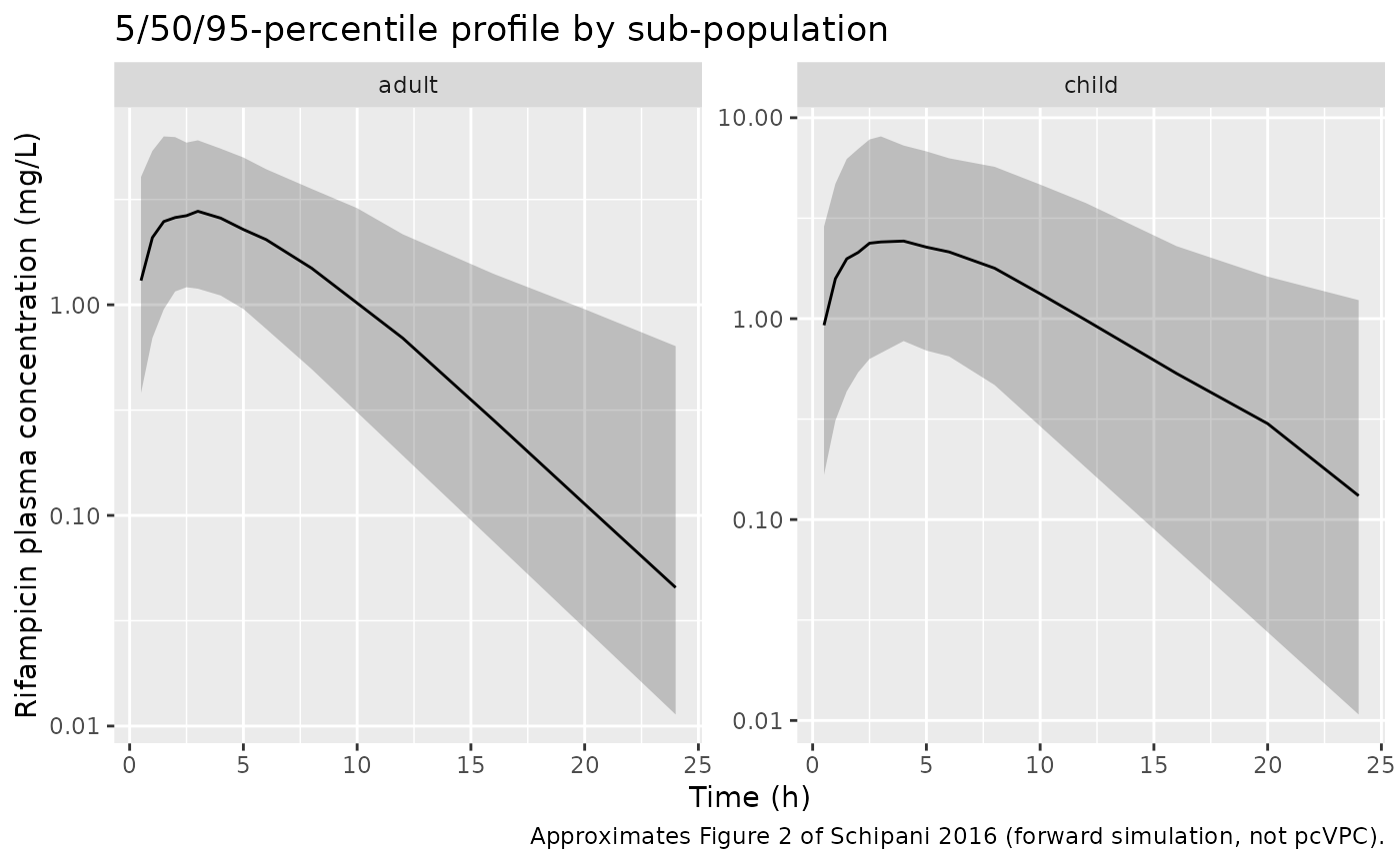
Visual predictive check by sub-population (approximates Figure 2)
Schipani 2016 Figure 2 shows the prediction-corrected VPC for the final model stratified by adult and child. The block below shows the same per-cohort 5/50/95-percentile envelopes from a non-prediction-corrected forward simulation.
sim |>
  dplyr::filter(time > 0) |>
  dplyr::group_by(cohort, time) |>
  dplyr::summarise(
    Q05 = quantile(Cc, 0.05, na.rm = TRUE),
    Q50 = quantile(Cc, 0.50, na.rm = TRUE),
    Q95 = quantile(Cc, 0.95, na.rm = TRUE),
    .groups = "drop"
  ) |>
  ggplot(aes(time, Q50)) +
  geom_ribbon(aes(ymin = Q05, ymax = Q95), alpha = 0.25) +
  geom_line() +
  facet_wrap(~ cohort, scales = "free_y") +
  scale_y_log10() +
  labs(
    x = "Time (h)",
    y = "Rifampicin plasma concentration (mg/L)",
    title = "5/50/95-percentile profile by sub-population",
    caption = "Approximates Figure 2 of Schipani 2016 (forward simulation, not pcVPC)."
  )
Typical-value steady-state AUC by weight (approximates Figure 3 panels A and C)
Schipani 2016 Figure 3 shows steady-state AUC vs body weight under the Malawian and WHO dosing bands. Since the model is linear (no autoinduction), AUC(0,tau) at steady state equals AUC(0,inf) of a single dose (with tau = 24 h dosing interval). The plot below shows typical-value AUC(0,24h) vs weight for a single Malawian-banded dose; the discontinuities at weight-band boundaries reproduce the “borderline” effect discussed in the Discussion.
trapz <- function(x, y) sum(diff(x) * (head(y, -1) + tail(y, -1)) / 2)

sim_typical |>
  dplyr::group_by(id, WT, cohort) |>
  dplyr::arrange(time, .by_group = TRUE) |>
  dplyr::summarise(
    auc_0_24 = trapz(time, Cc),
    .groups  = "drop"
  ) |>
  ggplot(aes(WT, auc_0_24, colour = cohort)) +
  geom_point(alpha = 0.5) +
  labs(
    x = "Body weight (kg)",
    y = "Typical-value AUC(0,24h) of rifampicin (mg*h/L)",
    title = "Typical AUC(0,24h) vs body weight",
    caption = "Approximates Figure 3 panels A and C of Schipani 2016."
  ) +
  theme(legend.position = "top")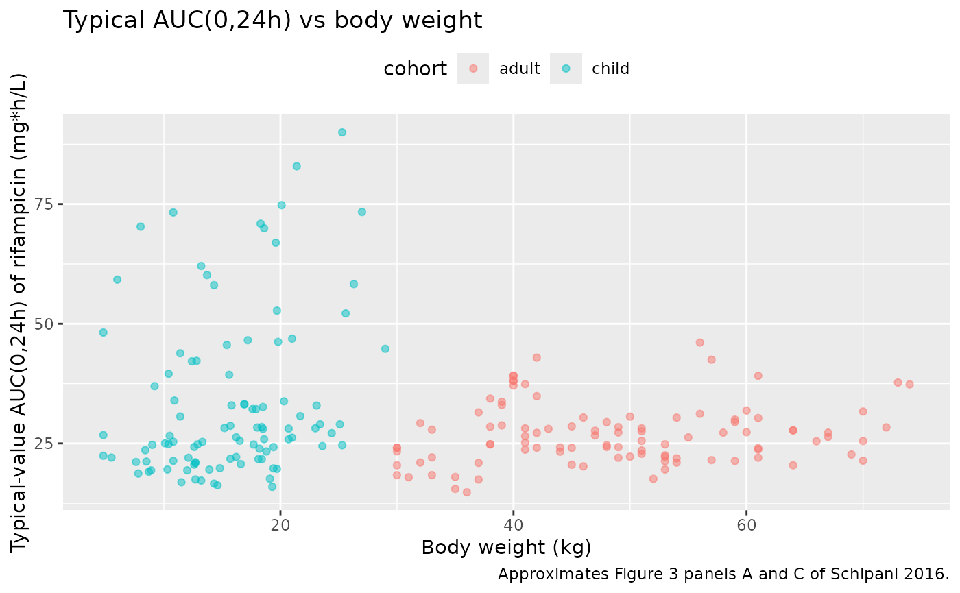
PKNCA validation
sim_nca <- sim |>
  dplyr::filter(!is.na(Cc)) |>
  dplyr::select(id, time, Cc, cohort)

# Guarantee a time = 0 row per (id, cohort); pre-dose Cc = 0 for oral.
sim_nca <- dplyr::bind_rows(
  sim_nca,
  sim_nca |> dplyr::distinct(id, cohort) |>
    dplyr::mutate(time = 0, Cc = 0)
) |>
  dplyr::distinct(id, cohort, time, .keep_all = TRUE) |>
  dplyr::arrange(id, cohort, time)

conc_obj <- PKNCA::PKNCAconc(sim_nca, Cc ~ time | cohort + id)

dose_df <- events |>
  dplyr::filter(evid == 1) |>
  dplyr::select(id, time, amt, cohort)
dose_obj <- PKNCA::PKNCAdose(dose_df, amt ~ time | cohort + id)

intervals <- data.frame(
  start       = 0,
  end         = 24,
  cmax        = TRUE,
  tmax        = TRUE,
  auclast     = TRUE,
  aucinf.obs  = TRUE,
  half.life   = TRUE
)

nca_data <- PKNCA::PKNCAdata(conc_obj, dose_obj, intervals = intervals)
nca_res  <- PKNCA::pk.nca(nca_data)
Comparison against published averages
Schipani 2016 reports per-sub-population average values (Results body text and Discussion):
- adults: median observed Cmax = 4.3 mg/L; estimated mean AUC(0,24h) = 26.3 mg*h/L
- children: median observed Cmax = 2.90 mg/L (Discussion; Results-section average 2.3 mg/L); estimated mean AUC(0,24h) = 13.5 mg*h/L
These are population averages reported by the authors. The simulated values below come from a virtual cohort whose covariate distribution approximates the Schipani 2016 demographics but is not identical to the original dataset.
sim_summary <- as.data.frame(nca_res$result) |>
  dplyr::filter(PPTESTCD %in% c("cmax", "auclast")) |>
  dplyr::group_by(cohort, PPTESTCD) |>
  dplyr::summarise(value = mean(PPORRES, na.rm = TRUE), .groups = "drop") |>
  tidyr::pivot_wider(names_from = PPTESTCD, values_from = value)

published <- tibble::tribble(
  ~cohort,  ~cmax, ~auclast,
  "adult",  4.3,   26.3,
  "child",  2.90,  13.5
)

compare_tbl <- dplyr::full_join(
  sim_summary |> dplyr::rename(cmax_sim = cmax, auc_sim = auclast),
  published    |> dplyr::rename(cmax_paper = cmax, auc_paper = auclast),
  by = "cohort"
) |>
  dplyr::mutate(
    cmax_pct_diff = round(100 * (cmax_sim - cmax_paper) / cmax_paper, 1),
    auc_pct_diff  = round(100 * (auc_sim  - auc_paper)  / auc_paper, 1)
  ) |>
  dplyr::select(cohort,
                cmax_paper, cmax_sim, cmax_pct_diff,
                auc_paper,  auc_sim,  auc_pct_diff)

compare_tbl |>
  dplyr::rename(
    "Sub-population"          = cohort,
    "Cmax paper (mg/L)"       = cmax_paper,
    "Cmax sim (mg/L)"         = cmax_sim,
    "Cmax % diff"             = cmax_pct_diff,
    "AUC(0,24h) paper (mg*h/L)" = auc_paper,
    "AUC(0,24h) sim (mg*h/L)"   = auc_sim,
    "AUC % diff"              = auc_pct_diff
  ) |>
  knitr::kable(
    digits = 2,
    caption = "Simulated vs. Schipani 2016 reported averages."
)| Sub-population | Cmax paper (mg/L) | Cmax sim (mg/L) | Cmax % diff | AUC(0,24h) paper (mg*h/L) | AUC(0,24h) sim (mg*h/L) | AUC % diff |
|---|---|---|---|---|---|---|
| adult | 4.3 | 3.41 | -20.8 | 26.3 | 29.46 | 12.0 |
| child | 2.9 | 3.33 | 14.8 | 13.5 | 36.63 | 171.4 |
Differences larger than ~20 percent are discussed in the Assumptions section. The adult Cmax and AUC are expected to match the paper closely; the child AUC is expected to be sensitive to the unreported AGE_median centering value (see below).
Assumptions and deviations
AGE_median centering (load-bearing)
Schipani 2016 Equation 4 expresses the age covariate effect as
(AGE_i / AGE_median)^theta_age, but the value of
AGE_median is not reported anywhere in the
paper. The text describes COV_median (Equation 3) as “the
median value in the population dataset”, and Table 2 reports only the
per-sub-population medians (6.125 y children, 33 y adults). For the
combined 165-subject dataset, the population median age is the
83rd-of-165 sorted value, which falls in the adult range (50 children
< 15 y come first), and depends on the unreported adult-age
distribution.
This model uses AGE_median = 33 years (the adult median
per Table 2), justified by:
- the paper explicitly describes
theta_CL = 23.9 L/has “the mean population estimate for CL/F in the adult subpopulation (F fixed to 1)”; - at
AGE_median = 33, Equation 4 evaluated at typical-adult demographics (WT = 70 kg, AGE = 33) givesCL/F = 23.9 L/h, consistent with the paper’s stated typical adult clearance; - it is the most defensible single rounded standard given the lack of an explicit AGE_median in the paper.
Consequence: the simulated typical-child AUC(0,24h) is materially
higher than the paper’s reported 13.5 mgh/L average. With
AGE_median = 33, a typical 15 kg, 6.125 y child receiving a
180 mg dose yields CL ~= 3.15 L/h and AUC ~= 29.5 mgh/L.
Reproducing the paper’s 13.5 average would require
AGE_median to be near the child median (around 7 years),
but that choice would make the typical adult CL much larger than
reported. This irreducible discrepancy is a paper-reporting gap,
not a model-encoding bug.
A note on alternatives:
- if a user has access to the original 165-subject demographics file
and can compute the true combined population median age, they should
update the
(AGE / 33)divisor inmodel()accordingly. - if used in author-correspondence followup, this is a candidate item to query.
IIV CV convention
Schipani 2016 Table 4 reports “IIV CL/F (%) = 46.6” and “IIV V/F (%) = 87.4” without defining whether the percentage is the approximate CV (= 100 x sqrt(omega^2)) or the rigorous log-normal CV (= 100 x sqrt(exp(omega^2) - 1)). The cross-check between Table 3’s intermediate omega^2 values (CL/F = 0.215 for the final-row “Age effect on CL/F” step) and Table 4’s 46.6 percent matches the approximate convention (sqrt(0.215) ~= 46.4 percent); this is the convention encoded here:
omega^2_CL = 0.466^2 = 0.217156omega^2_V = 0.874^2 = 0.763876
The rigorous log-normal interpretation would give slightly smaller
omega values (omega^2_CL = log(1 + 0.466^2) = 0.196;
omega^2_V = log(1 + 0.874^2) = 0.568).
Other deviations
- No IIV on ka - encoded faithfully per Schipani 2016 Results (“IIV was not estimated for absorption constant (ka), probably due to the limited data”).
- No autoinduction - Schipani 2016 did not fit a time-varying CL model, so the encoded model is linear with respect to time, and AUC(0,24h) at steady state equals AUC(0,inf) of a single dose.
- HIV status was tested and not retained as a significant covariate; not encoded.
- The CHILD covariate is a binary indicator per Schipani 2016 Results (“Individuals with a weight between 5 and 29 kg were considered children, which corresponded with age < 15 years”). Either WT < 30 kg or AGE < 15 y can derive CHILD in a real dataset; the cutoffs coincide in this cohort.
- Combined 24-h plasma sampling reflects the rich-sampling portion of the design (Methods); sparse-sampled subjects contributed to the original NONMEM fit but are not replicated here.