Magnesium sulfate (da Costa 2020)
Source:vignettes/articles/daCosta_2020_magnesiumSulfate.Rmd
daCosta_2020_magnesiumSulfate.RmdModel and source
- Citation: da Costa TX, Azeredo FJ, Ururahy MAG, da Silva Filho MA, Martins RR, Oliveira AG. Population Pharmacokinetics of Magnesium Sulfate in Preeclampsia and Associated Factors. Drugs R D 2020;20:257-266. doi:10.1007/s40268-020-00315-2
- Description: One-compartment population PK model of intravenous magnesium sulfate (MgSO4-7H2O) in pregnant women with preeclampsia, with an exponential serum-creatinine effect on clearance and an exponential body-weight effect on volume; no endogenous magnesium baseline (da Costa 2020).
- Article: https://doi.org/10.1007/s40268-020-00315-2
da Costa 2020 is a prospective observational population-PK study of
intravenous magnesium sulfate given by the Zuspan regimen (4 g over 30
min, then 1 g/h) to 109 Brazilian women with preeclampsia in a maternal
intensive care unit. The model is one-compartment with first-order
elimination, fitted in Monolix, with serum creatinine on clearance and
body weight on volume. Other magnesium sulfate models in this library
are Salinger_2013_magnesiumSulfate,
Easterling_2018_magnesium_sulfate,
Du_2019_magnesiumSulfate and
Deng_2024_magnesiumSulfate.
Read the Assumptions and deviations section before using this model. The covariate equation printed in the paper is unusable as written. The centring used here is supported by the paper’s own visual predictive check, as shown below. The model has no endogenous magnesium baseline, and it overpredicts the observed magnesium concentrations. The authors say so themselves.
Population
pop <- rxode2::rxode(readModelDb("daCosta_2020_magnesiumSulfate"))$population
#> ℹ parameter labels from comments will be replaced by 'label()'
str(pop, max.level = 1)
#> List of 12
#>  $ species       : chr "human"
#>  $ n_subjects    : int 109
#>  $ n_studies     : int 1
#>  $ n_observations: int 347
#>  $ age_range     : chr "mean 25.8 +/- 7.4 years"
#>  $ weight_range  : chr "mean 79.2 +/- 14.7 kg"
#>  $ sex_female_pct: num 100
#>  $ race_ethnicity: chr "not reported (Brazil)"
#>  $ disease_state : chr "Preeclampsia, third trimester (gestational age 35.2 +/- 4.2 weeks); maternal ICU. Baseline serum creatinine 0.7"| __truncated__
#>  $ dose_range    : chr "Zuspan regimen: 4 g MgSO4-7H2O IV over 30 min, then 1 g/h continuous IV infusion."
#>  $ regions       : chr "Brazil (Maternity School Januario Cicco, Natal)"
#>  $ notes         : chr "Prospective observational cohort, June 2016 - February 2018. Serum magnesium (colorimetric, Mann-Yoe) sampled b"| __truncated__
Baseline characteristics from da Costa 2020 Table 1 (n = 109, 347 serum magnesium concentrations, three to four per woman):
| Characteristic | Mean +/- SD |
|---|---|
| Age (years) | 25.8 +/- 7.4 |
| Body weight (kg) | 79.2 +/- 14.7 |
| Baseline magnesium (mg/dL) | 1.9 +/- 0.6 |
| Gestational age (weeks) | 35.2 +/- 4.2 |
| Baseline creatinine (mg/dL) | 0.7 +/- 0.3 |
Source trace
| Element | Value in model | Source |
|---|---|---|
| Structure: one compartment, first-order elimination, IV infusion | d/dt(central) <- -kel * central |
Methods 2.4 (infusion equation); Table 2 (1-cmt combined error selected) |
lcl |
log(1.38) L/h | Table 3, CL_pop; Results equation exp(0.3221 ...)
|
lvc |
log(13.3) L | Table 3, V_pop; Results equation exp(2.5878 ...)
|
e_creat_cl |
-0.0814 per mg/dL | Table 3, Beta_CL_creatinine_mg_dL |
e_wt_vc |
0.0752 per kg | Table 3, Beta_V_Weith_kg |
etalcl |
0.015^2 = 0.000225 | Table 3, Omega_CL = 0.015 (Monolix SD) |
etalvc |
0.404^2 = 0.163216 | Table 3, Omega_V = 0.404 (Monolix SD) |
addSd |
1.76 mg/dL | Table 3, residual error a |
propSd |
0.000552 | Table 3, residual error b |
| Covariate centring WT - 79.2, CREAT - 0.7 | cohort means | Table 1; supported by Figure 3 (see below) |
| Concentration unit mg/dL, no baseline | Cc <- central / vc / 10 |
Figure 3 axis; Methods 2.4 ‘No endogenous magnesium baseline adjustment’; Figure 1 predictions of 0 at pre-dose samples |
Units
Doses are entered as mg of elemental magnesium,
matching the other magnesium models in this library: multiply grams of
MgSO4-7H2O by 24.305 / 246.47 = 0.0986. The 4 g loading dose is 394.4 mg
Mg, and the 1 g/h maintenance infusion is 98.6 mg Mg/h. Cc
is in mg/dL of elemental magnesium, the unit of the paper’s VPC axis and
of the residual error a.
mg_per_g <- 24.305 / 246.47 * 1000
load_mg <- 4 * mg_per_g
rate_mg <- 1 * mg_per_g
c(load_mg = load_mg, rate_mg_per_h = rate_mg)
#>       load_mg rate_mg_per_h
#>     394.44963      98.61241
Covariate centring: the printed equation versus Figure 3
The Results print
V = exp(2.5878 + 0.0752 x weight (kg) + 0.404). Taken
literally, this adds the omega to the exponent and uses weight
uncentred. At the cohort-mean weight it gives V = 13.3 x exp(0.0752 x
79.2) = about 5,000 L. Magnesium would then be undetectable, so that
reading is not tenable. The Monolix beta must act on a centred
covariate. The paper does not print the centring value.
Figure 3, a VPC that simulates from the final model, settles the question. Its median prediction line starts at 0 at time 0 and rises through 1.3 mg/dL at 2 h and 3.4 mg/dL at 6 h. These medians were digitised from the figure by the maintainers. The rise is reproduced by the 1 g/h infusion alone, which also shows that the VPC dosing carried no loading dose. With that dosing, only centring at the cohort mean reproduces it. Centring at a rounded 70 kg makes the typical V twice as large and halves the early rise.
mod <- rxode2::rxode(readModelDb("daCosta_2020_magnesiumSulfate"))
#> ℹ parameter labels from comments will be replaced by 'label()'
mod_typ <- rxode2::zeroRe(mod)
stopifnot(is.null(mod$linCmt))

vpc_median <- data.frame(
  time = c(0, 2, 6, 12, 18, 28),
  fig3_median = c(0, 1.32, 3.43, 5.45, 3.75, 2.11)
)

typ_infusion <- function(wt, creat = 0.7, loading = FALSE) {
  ev <- rxode2::et(amt = rate_mg * 12, rate = rate_mg, cmt = "central")
  if (loading) {
    ev <- rxode2::et(amt = load_mg, dur = 0.5, cmt = "central") |>
      rxode2::et(amt = rate_mg * 12, rate = rate_mg, time = 0.5, cmt = "central")
  }
  ev <- rxode2::et(ev, vpc_median$time, cmt = "central")
  s <- rxode2::rxSolve(mod_typ, ev, params = data.frame(WT = wt, CREAT = creat))
  as.data.frame(s)$Cc
}

# Centring at 70 kg is equivalent, for the typical woman at 79.2 kg, to
# evaluating the 79.2-centred model at 79.2 + (79.2 - 70) kg.
centring <- vpc_median |>
  dplyr::mutate(
    `centred at 79.2 kg` = typ_infusion(79.2),
    `centred at 70 kg` = typ_infusion(79.2 + (79.2 - 70)),
    `79.2 kg, with 4 g load` = typ_infusion(79.2, loading = TRUE)
  )
#> ℹ omega/sigma items treated as zero: 'etalcl', 'etalvc'
#> ℹ omega/sigma items treated as zero: 'etalcl', 'etalvc'
#> ℹ omega/sigma items treated as zero: 'etalcl', 'etalvc'
knitr::kable(centring, digits = 2,
caption = "Typical-value Cc (mg/dL) under a 1 g/h infusion stopped at 12 h, against the Figure 3 median.")| time | fig3_median | centred at 79.2 kg | centred at 70 kg | 79.2 kg, with 4 g load |
|---|---|---|---|---|
| 0 | 0.00 | 0.00 | 0.00 | 0.00 |
| 2 | 1.32 | 1.34 | 0.71 | 3.50 |
| 6 | 3.43 | 3.31 | 1.91 | 4.74 |
| 12 | 5.45 | 5.09 | 3.31 | 5.86 |
| 18 | 3.75 | 2.73 | 2.43 | 3.35 |
| 28 | 2.11 | 0.97 | 1.44 | 1.19 |
rise <- centring |> dplyr::filter(time %in% c(2, 6))
stopifnot(
  # Centring at the cohort mean reproduces the published rise within 5%.
  all(abs(rise$`centred at 79.2 kg` / rise$fig3_median - 1) < 0.05),
  # A 70 kg centring misses it by more than 40%, as does a dosing record with
  # the 4 g load.
  all(abs(rise$`centred at 70 kg` / rise$fig3_median - 1) > 0.40),
  abs(rise$`79.2 kg, with 4 g load`[1] / rise$fig3_median[1] - 1) > 0.40
)
After 12 h the Figure 3 median declines more slowly than the typical-value solve (3.75 against 2.73 mg/dL at 18 h). The paper says the VPCs were stratified by infusion duration, so the pooled median after 12 h mixes women whose infusion was still running. The dosing history behind that part of the figure is not reported, so the decline is not used as a check.
Virtual cohort and Figure 3 replication
The cohort draws weight from N(79.2, 14.7) kg, truncated to 50-120 kg by rejection (the study excluded BMI > 40 kg/m^2). Creatinine is drawn log-normally with mean 0.7 and SD 0.3 mg/dL. Every woman receives the 1 g/h infusion without the loading dose, stopped at 12 h, to match the VPC dosing inferred above.
rxode2::rxSetSeed(20200708)
n_sub <- 200
draw_trunc <- function(n, mean, sd, lo, hi) {
  out <- numeric(0)
  while (length(out) < n) {
    x <- rnorm(n, mean, sd)
    out <- c(out, x[x >= lo & x <= hi])
  }
  out[seq_len(n)]
}
creat_sdlog <- sqrt(log(1 + (0.3 / 0.7)^2))
cohort <- data.frame(
  id = seq_len(n_sub),
  WT = draw_trunc(n_sub, 79.2, 14.7, 50, 120),
  CREAT = rlnorm(n_sub, log(0.7) - creat_sdlog^2 / 2, creat_sdlog)
)

obs_times <- sort(unique(c(seq(0, 28, by = 0.5), vpc_median$time)))
ev_vpc <- rxode2::et(amt = rate_mg * 12, rate = rate_mg, cmt = "central") |>
  rxode2::et(obs_times, cmt = "central") |>
  as.data.frame()
ev_vpc <- merge(cohort["id"], ev_vpc[, setdiff(names(ev_vpc), "id")], by = NULL) |>
  dplyr::left_join(cohort, by = "id") |>
  dplyr::arrange(id, time, dplyr::desc(evid))

sim_vpc <- rxode2::rxSolve(mod, ev_vpc, keep = c("WT", "CREAT")) |>
  as.data.frame()

vpc_sum <- sim_vpc |>
  dplyr::group_by(time) |>
  dplyr::summarise(
    p05 = quantile(sim, 0.05), p50 = quantile(sim, 0.50), p95 = quantile(sim, 0.95),
    .groups = "drop"
  )

ggplot(vpc_sum, aes(time)) +
  geom_ribbon(aes(ymin = p05, ymax = p95), fill = "steelblue", alpha = 0.25) +
  geom_line(aes(y = p50)) +
  geom_point(data = vpc_median, aes(time, fig3_median), colour = "firebrick", size = 2) +
  labs(x = "Time (h)", y = "Magnesium (mg/dL)",
       title = "Replicates Figure 3 of da Costa 2020",
       caption = "Line and ribbon: simulated median and 5th-95th centiles (with residual error).\nRed points: Figure 3 median prediction line, digitised by the maintainers.")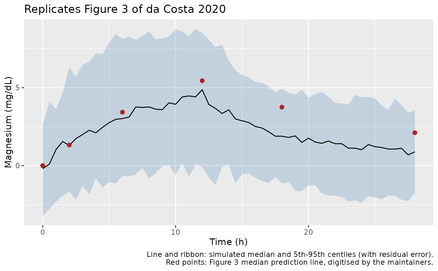
vpc_cmp <- sim_vpc |>
  dplyr::filter(time %in% c(2, 6)) |>
  dplyr::group_by(time) |>
  dplyr::summarise(ipred_median = median(ipredSim), .groups = "drop") |>
  dplyr::inner_join(vpc_median, by = "time")
knitr::kable(vpc_cmp, digits = 2)| time | ipred_median | fig3_median |
|---|---|---|
| 2 | 1.13 | 1.32 |
| 6 | 2.88 | 3.43 |
# Envelope check on the cohort's individual-prediction median. The residual
# error (additive SD 1.76 mg/dL) is larger than the 2 h median itself, so the
# median of the noisy simulated data is too unstable to gate on. The weight
# effect alone spreads V by a log-SD of about 1.1, so even the IPRED median of
# 200 women moves by about 10% between cohorts; the bound allows for that. The
# typical-value check above is the tight one.
stopifnot(all(abs(vpc_cmp$ipred_median / vpc_cmp$fig3_median - 1) < 0.35))
The simulated 5th-95th band at time 0 (about -3 to +3 mg/dL) is wider than the Figure 3 band (about -2.2 to +2.3 mg/dL). At time 0 only the additive error acts, so the published band implies an additive SD near 1.35 mg/dL against the tabulated a = 1.76. The Table 3 value is kept.
The weight effect is steep. exp(0.0752) = 1.078, so V rises 7.8% per kg, and one cohort SD of weight (14.7 kg) triples V. It is the dominant source of between-woman variability in the model, ahead of the 40% log-SD on V.
The clinical Zuspan regimen
A typical woman receives the protocol regimen (4 g over 30 min, then 1 g/h to 18 h). The paper reports an observed mean steady-state serum magnesium of 1.31 mmol/L (3.18 mg/dL, Discussion). That is total magnesium, and the baseline is 1.9 mg/dL (Table 1), so the drug-derived part is about 1.3 mg/dL.
ev_z <- rxode2::et(amt = load_mg, dur = 0.5, cmt = "central") |>
  rxode2::et(amt = rate_mg * 17.5, rate = rate_mg, time = 0.5, cmt = "central") |>
  rxode2::et(seq(0, 18, by = 0.25), cmt = "central")
sim_z <- rxode2::rxSolve(mod_typ, ev_z, params = data.frame(WT = 79.2, CREAT = 0.7)) |>
  as.data.frame()
#> ℹ omega/sigma items treated as zero: 'etalcl', 'etalvc'
css_typ <- rate_mg / exp(log(1.38)) / 10
knitr::kable(
  sim_z |> dplyr::filter(time %in% c(2, 6, 12, 18)) |> dplyr::select(time, Cc),
  digits = 2,
  caption = "Typical woman (79.2 kg, creatinine 0.7 mg/dL), drug-derived Cc (mg/dL)."
)| time | Cc |
|---|---|
| 2 | 3.50 |
| 6 | 4.74 |
| 12 | 5.86 |
| 18 | 6.45 |
c(model_css_mg_dL = css_typ, observed_drug_derived_mg_dL = 3.18 - 1.9)
#>             model_css_mg_dL observed_drug_derived_mg_dL
#>                    7.145827                    1.280000
The model’s steady state for a typical woman is 7.1 mg/dL of drug-derived magnesium. That is more than five times the observed drug-derived level. The overprediction is visible in the paper itself: in Figure 3 the observed concentrations at 12 h sit mostly below the median prediction line, and the Discussion notes that ‘the individual predicted concentrations are skewed towards being greater than the observed concentrations’. The packaged model reproduces the published parameters and does not correct this. Do not use it to predict absolute serum magnesium without that caveat.
PKNCA validation
NCA of the 4 g loading dose alone, typical values, at three weights.
The model is linear and one-compartment, so the NCA clearance, Dose /
AUCinf, must return the model’s CL, and the half-life must equal ln(2) V
/ CL. Cc is in mg/dL, so CL in L/h is Dose / (10 x
AUCinf).
wts <- c(60, 79.2, 100)
# Sample each weight for 12 typical half-lives. A fixed long grid drives the
# lightest woman (t1/2 about 1.6 h) far below the solver's absolute tolerance,
# and those noise-level points bias the lambda-z fit.
hl_typ <- log(2) * 13.3 * exp(0.0752 * (wts - 79.2)) / 1.38
ev_sd <- dplyr::bind_rows(lapply(seq_along(wts), function(i) {
  obs <- c(seq(0, 1, by = 0.05), seq(1.25, 12 * hl_typ[i], length.out = 400))
  rxode2::et(amt = load_mg, dur = 0.5, cmt = "central") |>
    rxode2::et(obs, cmt = "central") |>
    as.data.frame() |>
    dplyr::mutate(id = i)
})) |>
  dplyr::mutate(WT = wts[id], CREAT = 0.7, treatment = paste0("WT ", wts[id], " kg")) |>
  dplyr::arrange(id, time, dplyr::desc(evid))

sim_sd <- rxode2::rxSolve(mod_typ, ev_sd, keep = c("treatment", "WT")) |>
  as.data.frame()
#> ℹ omega/sigma items treated as zero: 'etalcl', 'etalvc'
#> Warning: multi-subject simulation without without 'omega'

conc_nca <- sim_sd |>
  dplyr::filter(!is.na(Cc)) |>
  dplyr::select(id, time, Cc, treatment)
stopifnot(all(tapply(conc_nca$time, conc_nca$id, min) == 0))
dose_nca <- ev_sd |>
  dplyr::filter(evid != 0) |>
  dplyr::select(id, time, amt, treatment)

conc_obj <- PKNCA::PKNCAconc(conc_nca, Cc ~ time | treatment + id)
dose_obj <- PKNCA::PKNCAdose(dose_nca, amt ~ time | treatment + id)
intervals <- data.frame(start = 0, end = Inf, cmax = TRUE, tmax = TRUE,
                        aucinf.obs = TRUE, half.life = TRUE)
nca_res <- PKNCA::pk.nca(PKNCA::PKNCAdata(conc_obj, dose_obj, intervals = intervals))

nca_wide <- as.data.frame(nca_res) |>
  dplyr::select(treatment, id, PPTESTCD, PPORRES) |>
  tidyr::pivot_wider(names_from = PPTESTCD, values_from = PPORRES) |>
  dplyr::inner_join(sim_sd |> dplyr::distinct(id, cl, vc), by = "id") |>
  dplyr::mutate(
    cl_nca = load_mg / (10 * aucinf.obs),
    hl_model = log(2) * vc / cl
  )

nca_wide |>
  dplyr::select(treatment, cmax, tmax, aucinf.obs, half.life, hl_model, cl_nca, cl) |>
  dplyr::rename("Group" = treatment, "Cmax (mg/dL)" = cmax, "Tmax (h)" = tmax,
                "AUCinf (mg*h/dL)" = aucinf.obs, "t1/2 NCA (h)" = half.life,
                "t1/2 model (h)" = hl_model, "CL NCA (L/h)" = cl_nca,
                "CL model (L/h)" = cl) |>
knitr::kable(digits = 3, caption = "PKNCA on the typical-value 4 g loading dose.")| Group | Cmax (mg/dL) | Tmax (h) | AUCinf (mg*h/dL) | t1/2 NCA (h) | t1/2 model (h) | CL NCA (L/h) | CL model (L/h) |
|---|---|---|---|---|---|---|---|
| WT 100 kg | 0.617 | 0.5 | 28.583 | 31.923 | 31.923 | 1.38 | 1.38 |
| WT 60 kg | 11.281 | 0.5 | 28.582 | 1.577 | 1.577 | 1.38 | 1.38 |
| WT 79.2 kg | 2.890 | 0.5 | 28.583 | 6.680 | 6.680 | 1.38 | 1.38 |
stopifnot(
  all(abs(nca_wide$cl_nca / nca_wide$cl - 1) < 0.01),
  all(abs(nca_wide$half.life / nca_wide$hl_model - 1) < 0.01)
)
The paper reports no NCA parameters (no Cmax, AUC or numeric half-life), so there is no published NCA table to compare against. The typical half-life at the cohort-mean weight is ln(2) x 13.3 / 1.38 = 6.7 h.
Assumptions and deviations
- Covariate centring (not printed). The Results equations print weight and creatinine uncentred, which makes V about 5,000 L at the cohort-mean weight. The model centres both on the Table 1 cohort means (79.2 kg, 0.7 mg/dL). The early rise of the Figure 3 VPC supports the weight centring: the typical-value solve centred at 79.2 kg matches the published median at 2 and 6 h within 5%, and a 70 kg centring misses it by more than 40%. The creatinine centring cannot be tested this way. Its effect is small (exp(-0.0814 x 0.7) = 0.945), and it is centred like weight for consistency.
-
Omega values added into the exponent. The Results
equations add 0.0151
- and 0.404 (V) inside
exp(). These are the Table 3 omegas. They are treated as the random-effect SDs they are, not as fixed shifts. The Table 3 value 0.015 is used for omega_CL; the equation’s 0.0151 agrees to rounding.
- and 0.404 (V) inside
- Omega scale. Monolix reports omega as the SD of the log-normal random effect, so the variances are 0.404^2 and 0.015^2. The Table 3 ‘CV’ column (19.3, 38.5) is the relative standard error of those estimates, not a between-subject CV. For omega_V, 0.0777 / 0.404 = 19.2%.
-
Residual error. Monolix’s combined model, sd = a +
b f, is encoded as nlmixr2
combined1(). With b = 0.000552 it is effectively additive at 1.76 mg/dL. The printed concentration equation,Mg = basalMg + (1.76 + 0.000552 x basalMg) x exp(CL/V x t), puts the residual-error parameters in place of an amplitude. It is not a usable structural equation, and the Methods infusion equation is used instead. -
Units. Dose is mg of elemental Mg and
Ccis mg/dL. The paper does not state its dataset’s dose unit. The Figure 3 check above fixes the scale: a 98.6 mg Mg/h infusion reproduces the published rise with the Table 3 CL and V. A dose in grams of MgSO4-7H2O would change it by a factor of about 10. -
No baseline. Following the paper (‘No endogenous
magnesium baseline adjustment was made to the model’),
Ccis drug-derived magnesium only. The fitted observations were total serum magnesium (baseline 1.9 +/- 0.6 mg/dL). The abstract’s ‘baseline magnesium concentration of 0.77 mmol/L (1.87 mg/dL)’ is not a parameter in Table 3. - Loading dose in the VPC. The Figure 3 median starts at 0 and has the shape of a pure 1 g/h infusion. With the 4 g load included, the 2 h value would be 3.5 mg/dL instead of 1.3 mg/dL. The paper does not say why the load is absent. The model file places no restriction on dosing.
- Overprediction. As shown above, the model’s steady state is more than five times the observed drug-derived magnesium. This is a property of the published estimates, which the authors acknowledge in their limitations.
- Inconsistent RSE column. The Table 3 ‘%’ column for V_pop and CL_pop (8.43, 17.4) is ten times the ratio of the printed SE to the estimate (0.84%, 1.7%). This does not affect the point estimates.
- No erratum was found in a EuropePMC search on 2026-09-27.