Tacrolimus meltdose (Martial 2021)
Source:vignettes/articles/Martial_2021_tacrolimus.Rmd
Martial_2021_tacrolimus.RmdModel and source
- Citation: Martial LC, Biewenga M, Ruijter BN, Keizer R, Swen JJ, van Hoek B, Moes DJAR. Population pharmacokinetics and genetics of oral meltdose tacrolimus (Envarsus) in stable adult liver transplant recipients. Br J Clin Pharmacol. 2021;87(11):4262-4272. doi:10.1111/bcp.14842
- Description: Two-compartment population pharmacokinetic model for once-daily oral meltdose tacrolimus (Envarsus) in stable adult liver transplant recipients converted from prolonged-release tacrolimus (Martial 2021). Delayed absorption uses the Savic transit-compartment input (1.58 transit compartments, mean transit time 3.39 h) feeding a first-order absorption compartment. Oral bioavailability is fixed at 0.23 with log-normal between-subject and between-occasion variability, and the peripheral volume is fixed at 500 L. Body weight enters by fixed allometry (exponent 0.75 on CL and Q, 1 on both volumes, reference 70 kg). Log-normal IIV on CL, Vc, Q and ka. Proportional residual error differs between venous whole-blood and dried-blood-spot samples.
- Article: https://doi.org/10.1111/bcp.14842 (open access, PMC8596620)
- Supplement: supplementary file S2 (InsightRX model verification
report), which prints the NONMEM control stream of the final model with
its final
$THETA,$OMEGAand$SIGMAestimates.
Population
Martial 2021 enrolled 55 stable adult liver transplant recipients at Leiden University Medical Center (Table 1): median age 57 years (range 21-70), median weight 81.5 kg (54-133), 34.5% female, 87% Caucasian, a median of 67 months after transplantation. All were on a stable prolonged-release tacrolimus (Advagraf) regimen and were converted to once-daily meltdose tacrolimus (Envarsus) at a 1:0.7 dose ratio; the median Envarsus dose was 2 mg/day (range 0.75-6). A full 24-h AUC was taken 2 weeks after conversion and an abbreviated AUC 3 months after conversion. The 0-6 h samples of the full AUC were venous whole blood and later samples were dried blood spots (DBS). Two patients were excluded for data inconsistencies, so 53 patients and 748 concentrations informed the model.
The same information is available programmatically:
str(rxode2::rxode(readModelDb("Martial_2021_tacrolimus"))$population)
#> ℹ parameter labels from comments will be replaced by 'label()'
#> Warning: some etas defaulted to non-mu referenced, possible parsing error: etaiov_fdepot_1, etaiov_fdepot_2, etaiov_fdepot_3
#> as a work-around try putting the mu-referenced expression on a simple line
#> List of 17
#>  $ species        : chr "human"
#>  $ n_subjects     : int 53
#>  $ n_enrolled     : int 55
#>  $ n_observations : int 748
#>  $ age_range      : chr "21-70 years"
#>  $ age_median     : chr "57 years"
#>  $ weight_range   : chr "54-133 kg"
#>  $ weight_median  : chr "81.5 kg"
#>  $ height_median  : chr "175 cm (range 151-189 cm)"
#>  $ sex_female_pct : num 34.5
#>  $ race_ethnicity : chr "Caucasian 87% (48 of 55); others not stratified."
#>  $ disease_state  : chr "Stable adult liver transplant recipients at least 6 months after transplantation (median 67 months, range 6-240"| __truncated__
#>  $ dose_range     : chr "Once-daily oral Envarsus, median 2 mg (range 0.75-6 mg) (Table 1), adjusted to individual whole-blood trough targets."
#>  $ regions        : chr "The Netherlands (Leiden University Medical Center)."
#>  $ co_medication  : chr "Mycophenolate mofetil 49%, prednisone 9.1%, everolimus 5.5%, sirolimus 3.6%, azathioprine 3.6% (Table 1)."
#>  $ sampling_design: chr "Full AUC (0, 1, 2, 3, 4, 6, 8, 12, 24 h) 2 weeks after conversion, abbreviated AUC (0, 4, 8, 12 h) 3 months aft"| __truncated__
#>  $ notes          : chr "Baseline demographics from Martial 2021 Table 1 (all 55 enrolled). Two patients were excluded from the PK analy"| __truncated__
Source trace
Final-model estimates are from Martial 2021 Table 3. The variances
and the model code are from the NONMEM control stream in supplementary
file S2, whose $THETA values match Table 3 and whose
$OMEGA / $SIGMA values reproduce every Table 3
CV% as 100 * sqrt(variance).
| Equation / parameter | Value | Source location |
|---|---|---|
lcl (CL, 70 kg) |
log(3.27) L/h | Table 3 ‘CL/F’; S2 $THETA(1)
|
lvc (Vc, 70 kg) |
log(94.9) L | Table 3 ‘V1/F’; S2 $THETA(2)
|
lq (Q, 70 kg) |
log(9.62) L/h | Table 3 ‘Q/F’; S2 $THETA(4)
|
lvp (Vp, 70 kg) |
fixed(log(500)) L | Table 3 ‘V2/F (fixed)’; Results 3.2; S2 $THETA(5)
FIX |
lka |
log(2.97) 1/h | Table 3 ‘Ka’ (S2 prints 2.96) |
lmtt |
log(3.39) h | Table 3 ‘MTT’; S2 $THETA(7)
|
lntr |
log(1.58) | Table 3 ‘Ntrans’; S2 $THETA(8)
|
lfdepot |
fixed(log(0.23)) | Table 3 ‘F (fixed)’; S2 $THETA(6) FIX |
e_wt_cl_q, e_wt_vc_vp
|
fixed 0.75, fixed 1 | Methods 2.6; S2 $PK
|
etalcl |
0.116 | Table 3 34%; S2 $OMEGA
|
etalvc |
1.99 | Table 3 141%; S2 $OMEGA
|
etalq |
0.0571 | Table 3 24%; S2 $OMEGA
|
etalka |
3.02 | Table 3 174%; S2 $OMEGA
|
etalfdepot |
0.131 | Table 3 36%; S2 $OMEGA
|
etaiov_fdepot_1..3 |
0.0388 (2, 3 SAME) | Table 3 ‘IOV F (block)’ 19.7%; S2 $OMEGA BLOCK(1) +
SAME
|
propSd |
0.10536 | Table 3 ‘Whole blood’ 10.5%; S2 $SIGMA 0.0111 |
propSdDbs |
0.24900 | Table 3 ‘DBS’ 24.9%; S2 $SIGMA 0.062 |
ktr = (ntr + 1) / mtt |
n/a | S2 $PK KTR
|
lnfac (Stirling log(ntr!)) |
n/a | S2 $PK LNFAC
|
d/dt(depot) Savic input |
n/a | S2 $DES DADT(1)
|
d/dt(central), d/dt(peripheral1)
|
n/a | S2 $DES DADT(2), DADT(3)
|
| Weight scaling of CL, Vc, Q, Vp | n/a | Methods 2.6; S2 $PK
|
Cc = 1000 * central / vc (ug/L) |
n/a | S2 $ERROR scaling S2 = V2/1000
|
| Matrix-specific proportional error | n/a | Methods 2.4; S2 $ERROR
|
Virtual cohort
The observed data are not public. The cohort below has 200 subjects given the median Envarsus dose (2 mg once daily), with body weight drawn log-normally around the Table 1 median of 81.5 kg and truncated to the observed 54-133 kg range. Patients in the study had been on tacrolimus for years before the first AUC, so every subject is dosed for 90 days before the observed interval. The terminal half-life of the typical subject is about 157 h, so 90 days is more than 13 half-lives and the last interval is at steady state. All records are occasion 1 (the first full AUC), and the sampling matrix follows the study design: venous whole blood up to 6 h after the dose and DBS afterwards.
set.seed(2021)
n_sub <- 200
t_ss <- 24 * 90
obs_tad <- c(0, 0.5, 1, 1.5, 2, 3, 4, 5, 6, 7, 8, 10, 12, 16, 20, 24)

make_cohort <- function(n, dose, id_offset = 0L) {
  subj <- tibble(
    id = id_offset + seq_len(n),
    WT = pmin(pmax(exp(rnorm(n, log(81.5), 0.2)), 54), 133)
  )
  doses <- tidyr::crossing(subj, time = seq(0, t_ss, by = 24)) |>
    mutate(evid = 1L, amt = dose, cmt = "depot")
  obs <- tidyr::crossing(subj, time = t_ss + obs_tad) |>
    mutate(evid = 0L, amt = 0, cmt = "central")
  bind_rows(doses, obs) |>
    mutate(
      OCC = 1L,
      SAMPLE_DBS = as.integer(evid == 0L & (time - t_ss) > 6),
      treatment = paste0(dose, " mg QD")
    ) |>
    arrange(id, time, desc(evid))
}

events <- make_cohort(n_sub, dose = 2)
stopifnot(!anyDuplicated(unique(events[, c("id", "time", "evid")])))
Simulation
mod <- rxode2::rxode(readModelDb("Martial_2021_tacrolimus"))
#> ℹ parameter labels from comments will be replaced by 'label()'
#> Warning: some etas defaulted to non-mu referenced, possible parsing error: etaiov_fdepot_1, etaiov_fdepot_2, etaiov_fdepot_3
#> as a work-around try putting the mu-referenced expression on a simple line
rxode2::rxSetSeed(2021)
sim <- rxode2::rxSolve(mod, events = events, keep = c("treatment", "WT")) |>
  as.data.frame() |>
  mutate(tad = time - t_ss)
# Guard against a transit input that silently delivers no drug.
stopifnot(max(sim$Cc) > 1)
Typical-value mass balance
At steady state the AUC over one dosing interval equals
F * Dose / CL. The estimation model computes
log(ntr!) with the Stirling approximation rather than
lgamma(ntr + 1), so the transit input delivers
exp(lgamma(ntr + 1) - lnfac) times the bioavailable dose,
which is 1.0007 at ntr = 1.58. This deterministic check
confirms the dose, the bioavailability, the transit input and the
clearance are wired together correctly.
typ <- rxode2::zeroRe(mod)
#> Warning: No sigma parameters in the model
#> Warning: some etas defaulted to non-mu referenced, possible parsing error: etaiov_fdepot_1, etaiov_fdepot_2, etaiov_fdepot_3
#> as a work-around try putting the mu-referenced expression on a simple line
ev_typ <- bind_rows(
  tibble(time = seq(0, t_ss, by = 24), evid = 1L, amt = 2, cmt = "depot"),
  tibble(time = t_ss + seq(0, 24, by = 0.05), evid = 0L, amt = 0, cmt = "central")
) |>
  mutate(id = 1L, WT = 70, OCC = 1L, SAMPLE_DBS = 0L) |>
  arrange(time, desc(evid))
sim_typ <- rxode2::rxSolve(typ, events = ev_typ) |>
  as.data.frame() |>
  mutate(tad = time - t_ss) |>
  filter(tad >= 0)
#> ℹ omega/sigma items treated as zero: 'etalcl', 'etalvc', 'etalq', 'etalka', 'etalfdepot', 'etaiov_fdepot_1', 'etaiov_fdepot_2', 'etaiov_fdepot_3'

auc_tau <- with(sim_typ, sum(diff(tad) * (head(Cc, -1) + tail(Cc, -1)) / 2))
ntr <- 1.58
lnfac <- log(2.5066) + (ntr + 0.5) * log(ntr) - ntr + log(1 + 1 / (12 * ntr))
expected_ratio <- exp(lgamma(ntr + 1) - lnfac)
ratio <- auc_tau * 3.27 / (0.23 * 2 * 1000)

typ_summary <- tibble(
  quantity = c(
    "AUC0-24 at steady state (ug*h/L)",
    "AUC0-24 * CL / (F * Dose)",
    "Expected ratio exp(lgamma(ntr+1) - lnfac)",
    "Trough C0 (ug/L)",
    "Cmax (ug/L)",
    "Tmax (h)"
  ),
  value = c(
    auc_tau, ratio, expected_ratio, sim_typ$Cc[1], max(sim_typ$Cc),
    sim_typ$tad[which.max(sim_typ$Cc)]
  )
)
knitr::kable(typ_summary, digits = 4,
caption = "Typical 70 kg subject, 2 mg once daily at steady state.")| quantity | value |
|---|---|
| AUC0-24 at steady state (ug*h/L) | 140.7657 |
| AUC0-24 * CL / (F * Dose) | 1.0007 |
| Expected ratio exp(lgamma(ntr+1) - lnfac) | 1.0007 |
| Trough C0 (ug/L) | 4.7155 |
| Cmax (ug/L) | 7.3670 |
| Tmax (h) | 5.7000 |
# Deterministic: trapezoid error on a 0.05 h grid is far below 1e-3.
stopifnot(abs(ratio - expected_ratio) < 1e-3)
The typical 70 kg subject on the median 2 mg dose has a steady-state AUC0-24 of about 141 ug*h/L. That is 2% below the Table 1 cohort median of 144 ug*h/L. It also matches the Discussion’s statement that the apparent clearance is 3.27 / 0.23 = 14.2 L/h, because 2000 ug / 14.2 L/h = 141 ug*h/L.
Replicate published figures
Figure 2 and Figure 5: concentration-time profile at the first full AUC
# Replicates Figure 2 (observed profiles at the first full AUC) and the
# percentile bands of Figure 5 (prediction-corrected VPC) of Martial 2021.
vpc <- sim |>
  group_by(tad) |>
  summarise(
    Q05 = quantile(Cc, 0.05),
    Q50 = quantile(Cc, 0.50),
    Q95 = quantile(Cc, 0.95),
    .groups = "drop"
  )
ggplot(vpc, aes(tad, Q50)) +
  geom_ribbon(aes(ymin = Q05, ymax = Q95), alpha = 0.25, fill = "steelblue") +
  geom_line(linewidth = 1) +
  scale_x_continuous(breaks = seq(0, 24, 4)) +
  labs(
    x = "Time after dose (h)",
    y = "Whole-blood tacrolimus (ug/L)",
    title = "Simulated steady-state profile, 2 mg once daily",
    caption = "Median and 5th-95th percentiles. Replicates Figures 2 and 5 of Martial 2021."
  )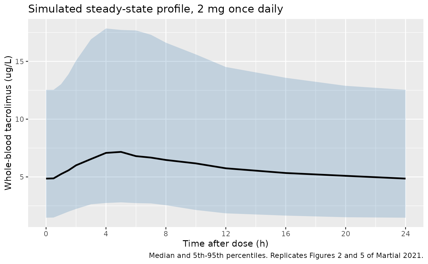
The simulated median rises from 4.9 ug/L before the dose to 7.2 ug/L at 5 h and falls back by 24 h. In the Figure 5 VPC the observed median rises from about 4.5 to about 7 ug/L, with the 5th and 95th percentile lines near 2 and 12-20 ug/L. The simulated bands are close to those lines and to the spread of the individual profiles in Figure 2.
Figure 6 (first panel): AUC0-24 versus trough concentration
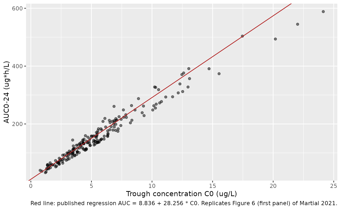
Martial 2021 regressed the model-based AUC0-24 on the trough
concentration and reported AUC = 8.836 + 28.256 * C0
(Results 3.3). The cohort below uses one dose level, while the study
population’s doses ranged from 0.75 to 6 mg. The comparison therefore
uses the per-subject ratio AUC0-24 / C0, which does not depend on dose.
At the published median AUC of 144 ug*h/L the regression implies C0 =
4.78 ug/L and a ratio of 30.1.
# Replicates the first panel of Figure 6 of Martial 2021.
per_subj <- sim |>
  group_by(id) |>
  summarise(
    C0 = Cc[tad == 0],
    auc = sum(diff(tad) * (head(Cc, -1) + tail(Cc, -1)) / 2),
    .groups = "drop"
  )
ggplot(per_subj, aes(C0, auc)) +
  geom_point(alpha = 0.5) +
  geom_abline(intercept = 8.836, slope = 28.256, colour = "firebrick") +
  labs(
    x = "Trough concentration C0 (ug/L)",
    y = "AUC0-24 (ug*h/L)",
    caption = "Red line: published regression AUC = 8.836 + 28.256 * C0. Replicates Figure 6 (first panel) of Martial 2021."
  )
c0_published <- (144 - 8.836) / 28.256
ratio_published <- 144 / c0_published
ratio_sim <- median(per_subj$auc / per_subj$C0)
c(published = ratio_published, simulated = ratio_sim)
#> published simulated
#>  30.10316  29.20138

# Centre of the cohort distribution, robust to which subjects land in the
# tails (median of 200 ratios; the values seen while authoring were 28-29).
stopifnot(abs(ratio_sim / ratio_published - 1) < 0.15)
PKNCA validation
sim_nca <- sim |>
  filter(!is.na(Cc)) |>
  select(id, treatment, time = tad, Cc)

conc_obj <- PKNCA::PKNCAconc(sim_nca, Cc ~ time | treatment + id)
dose_df <- sim_nca |>
  distinct(id, treatment) |>
  mutate(time = 0, amt = 2)
dose_obj <- PKNCA::PKNCAdose(dose_df, amt ~ time | treatment + id)

intervals <- data.frame(
  start = 0, end = 24,
  auclast = TRUE, cmax = TRUE, tmax = TRUE, cmin = TRUE
)
nca_res <- PKNCA::pk.nca(PKNCA::PKNCAdata(conc_obj, dose_obj, intervals = intervals))
summary(nca_res)
#>  start end treatment   N    auclast        cmax        cmin              tmax
#>      0  24   2 mg QD 200 136 [62.0] 7.31 [61.1] 4.66 [68.9] 6.00 [3.00, 12.0]
#>
#> Caption: auclast, cmax, cmin: geometric mean and geometric coefficient of variation; tmax: median and range; N: number of subjects
Comparison against published NCA
Martial 2021 reports only the cohort median Envarsus AUC0-24 (Table 1: 144 ug*h/L, range 25-323).
published <- tibble::tribble(
  ~treatment, ~auclast,
  "2 mg QD", 144
)
cmp <- nlmixr2lib::ncaComparisonTable(
  simulated = nca_res,
  reference = published,
  by = "treatment",
  units = c(auclast = "ug*h/L"),
  tolerance_pct = 20
)
knitr::kable(cmp, caption = "Simulated vs. published steady-state AUC0-24. * differs from reference by >20%.")| NCA parameter | treatment | Reference | Simulated | % diff |
|---|---|---|---|---|
| AUClast (ug*h/L) | 2 mg QD | 144 | 138 | -4.5% |
The simulated cohort median AUC0-24 is 138 ug*h/L, -4% from the
published median. This is not a like-for-like comparison. The cohort’s
median weight is 81.5 kg, and at that weight the typical clearance is
3.27 * (81.5 / 70)^0.75 = 3.67 L/h, which puts the typical
AUC0-24 at 125 ug*h/L. The published median comes from patients whose
doses were titrated to trough targets, so each patient’s dose tracks
their own clearance, and a cohort given one fixed dose does not
reproduce that. The median of 200 subjects with this much
between-subject variability also moves by several percent from one
random draw to the next. The 70 kg typical-value check above is the
like-for-like comparison.
Assumptions and deviations
-
CL, V1, Q and V2 are systemic values, not apparent.
Table 3 labels them CL/F, V1/F, Q/F and V2/F. However, the control
stream in supplementary file S2 applies the fixed F = 0.23 to the dose
inside the transit input, the Methods define the model AUC as
DOSE * F / CL, and the Discussion back-calculates the apparent clearance as 3.27 / 0.23 = 14.2 L/h. The model applies F = 0.23 in the same way. The typical-value AUC check above reproduces the Table 1 median AUC only under this reading; reading 3.27 L/h as CL/F would give an AUC about 4.3-fold higher. -
Omega and sigma scale. Table 3 prints only CV%. The
S2 control stream prints the variances, and
100 * sqrt(variance)reproduces every Table 3 CV% (for example 0.116 gives 34% and 1.99 gives 141%), so the variances are used as printed. - Ka. Table 3 prints 2.97 1/h and the S2 control stream prints 2.96 1/h. The Table 3 value is used.
-
Stirling approximation. The estimation model
computes the log factorial in the Savic transit input with the Stirling
approximation (S2
LNFAC). The model keeps that expression, so the transit input delivers 1.0007 times the bioavailable dose. That is how the published parameters were estimated. TheX = 0.00001offsets inside the logarithms of the S2$DESare numerical guards and are not reproduced. -
Occasions. The Methods define three occasions, one
per AUC measurement, and Table 3 prints three IOV shrinkages. The model
therefore uses
OCC= 1-3. The S2 verification stream instead switches occasions by 24-h clock windows and carries four IOV etas. That scheme belongs to the dosing-software implementation and was not used to estimate the model. The Results say the IOV “omega block” allowed correlation between occasions. The S2 stream codes it as$OMEGA BLOCK(1)followed bySAME, i.e. one shared variance and no correlation, and that is what is encoded. Records with any otherOCCvalue carry no IOV. -
Sampling matrix.
SAMPLE_DBS = 1selects the DBS residual error. The reference level (0) is venous whole blood, because tacrolimus is measured in whole blood and the study had no plasma samples. No systematic DBS-to-venous conversion factor was estimated. - Transit input restarts at each dose. The Savic input is driven by the time since the most recent dose, as in the source model. With MTT = 3.39 h and a 24-h dosing interval, essentially none of a dose is still in transit when the next dose is given.
-
Covariates screened but not retained (hematocrit,
recipient and donor CYP3A5*3 and CYP3A4*22, and the IL-6, IL-10 and
IL-18 genotypes) are documented in the model’s
covariatesDataExcludedmetadata and are not in the model. - Virtual cohort. Everyone receives the median 2 mg dose, and weight is log-normal (SD 0.2 on the log scale) around 81.5 kg, truncated to 54-133 kg. The study’s titrated doses are not modelled.
- No erratum or correction notice for this article was found as of 2026-09-29.