Roxadustat (Takada 2022)
Source:vignettes/articles/Takada_2022_roxadustat.Rmd
Takada_2022_roxadustat.RmdModel and source
- Citation: Takada A, Shibata T, Shiga T, Groenendaal-van de Meent D, Komatsu K. Population pharmacokinetics of roxadustat in Japanese dialysis-dependent chronic kidney disease patients with anaemia. Br J Clin Pharmacol. 2022;88(2):787-797. doi:10.1111/bcp.15023
- Description: Two-compartment population PK model with first-order absorption and lag time for oral roxadustat (HIF-prolyl hydroxylase inhibitor) in Japanese dialysis-dependent chronic kidney disease patients with anaemia, on haemodialysis or peritoneal dialysis (Takada 2022). Age >= 65 years lowers CL/F; five concomitant phosphate binders (sevelamer hydrochloride/bixalomer, calcium carbonate, lanthanum carbonate, ferric citrate, sucroferric oxyhydroxide) each lower the relative bioavailability, with an additional decrease when phosphate binders were taken without time separation (phase II study).
- Article: https://doi.org/10.1111/bcp.15023 (open access; PMC9292185)
Population
Takada et al. pooled 367 Japanese patients (256 male, 111 female) with anaemia of dialysis-dependent chronic kidney disease from four Astellas studies of oral roxadustat given three times weekly (Table 1): the phase II haemodialysis study 1517-CL-0304 (n = 92, after an ESA washout) and three phase III studies, 1517-CL-0308 (haemodialysis, ESA-untreated, n = 74), 1517-CL-0307 (haemodialysis, conversion from ESA, n = 145) and 1517-CL-0302 (peritoneal dialysis, n = 56). Mean (SD) age was 64.4 (10.9) years, weight 59.5 (11.8) kg and BMI 22.8 (3.5) kg/m^2 (Table 3). Initial doses of 50, 70 or 100 mg were titrated on haemoglobin to 20-250 mg. Sparse samples (1285 concentrations) were taken at study visits at any time relative to dose and dialysis.
Phosphate binders were common: 82.0% of patients took at least one during the study (Table 3): calcium carbonate 47.7%, lanthanum carbonate 37.9%, sevelamer hydrochloride or bixalomer 21.5%, ferric citrate 16.1% and sucroferric oxyhydroxide 4.6%. The phase III protocols required roxadustat to be taken at least 1 hour before or after a phosphate binder; the phase II study did not.
The same information is available programmatically via
readModelDb("Takada_2022_roxadustat")()$population.
Source trace
Every ini() value in
inst/modeldb/specificDrugs/Takada_2022_roxadustat.R carries
an in-file comment pointing at its source. All final estimates come from
Table 4 of the article.
| Component | Value | Source |
|---|---|---|
| Two-compartment disposition, first-order absorption with lag time | – | Results 3.2; Conclusion |
Log-normal IIV, P_i = theta * exp(eta_i)
|
– | Methods 2.4 equation |
Categorical covariate model
P_i = theta1 * theta2^(0 or 1)
|
– | Methods 2.5 equation |
| CL/F | 0.923 L/h | Table 4 |
| Vc/F | 14.6 L | Table 4 |
| ka | 0.63 1/h | Table 4 |
| Q/F | 0.134 L/h | Table 4 |
| Vp/F | 2.89 L | Table 4 |
| ALAG1 | 0.287 h | Table 4 |
| Age >= 65 y on CL/F | 0.792 | Table 4; Results 3.4 |
| Sevelamer/bixalomer (SBUSE) on F1 | 0.744 | Table 4 |
| Calcium carbonate (CUSE) on F1 | 0.931 | Table 4 |
| Lanthanum carbonate (LUSE) on F1 | 0.969 | Table 4 |
| Ferric citrate (FUSE) on F1 | 0.744 | Table 4 |
| Sucroferric oxyhydroxide (SCUSE) on F1 | 0.837 | Table 4 |
| No time separation of PBs in phase II on F1 | 0.935 | Table 4 and its footnote |
| IIV CL/F | 41.7% -> omega^2 = 0.1739 | Table 4 (see “IIV scale” below) |
| IIV Vc/F | 22.0% -> omega^2 = 0.0484 | Table 4 |
| IIV ka | 184.1% -> omega^2 = 3.389 | Table 4 |
Combined residual error
W = sqrt((IPRED * theta_prop)^2 + theta_add^2)
|
– | Methods 2.4 equation |
| Proportional residual SD | 0.439 | Table 4 |
| Additive residual SD | 1.88 ng/mL | Table 4 |
Dose mg, V in L -> Cc = 1000 * central / vc in
ng/mL |
– | Methods 2.2 (ng/mL assay) |
IIV scale
Table 4 reports IIV as “%CV” without saying how it was computed from
omega^2. The printed 95% confidence intervals settle it:
they are omega^2 +/- 1.96 * SE (with SE = RSE x
omega^2) back-transformed by a square root, so the reported
percentage is 100 * sqrt(omega^2). The two readings are
nearly indistinguishable for the moderate CL/F and Vc/F rows, but the
wide ka row separates them: only the sqrt(omega^2) reading
reproduces its 154.2-209.8% interval.
iiv <- data.frame(
  parameter = c("CL/F", "Vc/F", "ka"),
  cv = c(0.417, 0.220, 1.841),
  rse = c(0.096, 0.503, 0.152),
  lo_pub = c(0.376, 0.026, 1.542),
  hi_pub = c(0.455, 0.310, 2.098)
)
iiv <- iiv |>
  dplyr::mutate(
    # Reading A: %CV = sqrt(omega^2)
    om2_a = cv^2,
    lo_a = sqrt(om2_a * (1 - 1.96 * rse)),
    hi_a = sqrt(om2_a * (1 + 1.96 * rse)),
    # Reading B: %CV = sqrt(exp(omega^2) - 1)
    om2_b = log(1 + cv^2),
    lo_b = sqrt(exp(om2_b * (1 - 1.96 * rse)) - 1),
    hi_b = sqrt(exp(om2_b * (1 + 1.96 * rse)) - 1)
  )
iiv |>
  dplyr::transmute(
    Parameter = parameter,
    "Published 95% CI" = sprintf("%.1f-%.1f%%", 100 * lo_pub, 100 * hi_pub),
    "sqrt(omega^2) reading" = sprintf("%.1f-%.1f%%", 100 * lo_a, 100 * hi_a),
    "log(1 + CV^2) reading" = sprintf("%.1f-%.1f%%", 100 * lo_b, 100 * hi_b)
  ) |>
knitr::kable()| Parameter | Published 95% CI | sqrt(omega^2) reading | log(1 + CV^2) reading |
|---|---|---|---|
| CL/F | 37.6-45.5% | 37.6-45.5% | 37.3-45.8% |
| Vc/F | 2.6-31.0% | 2.6-31.0% | 2.6-31.4% |
| ka | 154.2-209.8% | 154.3-209.7% | 135.1-241.2% |
# The sqrt(omega^2) reading reproduces every published bound to within the
# table's rounding; the log(1 + CV^2) reading misses the wide ka row by >15
# percentage points.
stopifnot(
  all(abs(iiv$lo_a - iiv$lo_pub) < 0.002),
  all(abs(iiv$hi_a - iiv$hi_pub) < 0.002),
  abs(iiv$hi_b[3] - iiv$hi_pub[3]) > 0.15
)
Covariate effects on exposure (Figure 4)
The paper summarises each covariate as the percentage change in
roxadustat AUCinf, where AUCinf = Dose / (CL/F) with CL/F
adjusted for the covariates (Methods 2.7). Because each phosphate binder
acts on F1, the AUCinf change is F1 factor - 1; age acts on
CL/F, so AUCinf changes by 1/0.792 - 1 = +26.3% (Results
3.4). The check below solves the packaged model for a typical patient
(no IIV) after a single 100 mg dose, computes AUCinf with PKNCA for each
covariate setting, and compares the ratio with Figure 4.
mod <- rxode2::rxode2(readModelDb("Takada_2022_roxadustat"))
#> ℹ parameter labels from comments will be replaced by 'label()'
mod_typ <- rxode2::zeroRe(mod)

no_cov <- data.frame(
  AGE = 60,
  CONMED_SEVELAMER_BIXALOMER = 0,
  CONMED_CALCIUM_CARBONATE = 0,
  CONMED_LANTHANUM_CARBONATE = 0,
  CONMED_FERRIC_CITRATE = 0,
  CONMED_SUCROFERRIC_OXYHYDROXIDE = 0,
  STUDY_PHASE2 = 0
)

scenarios <- list(
  "Reference" = no_cov,
  "Age >= 65 y" = dplyr::mutate(no_cov, AGE = 70),
  "Sevelamer/bixalomer" = dplyr::mutate(no_cov, CONMED_SEVELAMER_BIXALOMER = 1),
  "Sucroferric oxyhydroxide" = dplyr::mutate(no_cov, CONMED_SUCROFERRIC_OXYHYDROXIDE = 1),
  "Ferric citrate" = dplyr::mutate(no_cov, CONMED_FERRIC_CITRATE = 1),
  "Calcium carbonate" = dplyr::mutate(no_cov, CONMED_CALCIUM_CARBONATE = 1),
  "Lanthanum carbonate" = dplyr::mutate(no_cov, CONMED_LANTHANUM_CARBONATE = 1),
  # The phase II factor applies only on top of a coadministered binder;
  # compare calcium carbonate without vs with time separation.
  "Calcium carbonate, no time separation" =
    dplyr::mutate(no_cov, CONMED_CALCIUM_CARBONATE = 1, STUDY_PHASE2 = 1),
  # STUDY_PHASE2 alone (no binder) must not change exposure.
  "Phase II, no binder" = dplyr::mutate(no_cov, STUDY_PHASE2 = 1)
)

obs_times <- c(0, seq(0.25, 12, by = 0.25), seq(13, 48, by = 1), seq(54, 480, by = 6))
fig4_events <- dplyr::bind_rows(lapply(seq_along(scenarios), function(i) {
  covs <- scenarios[[i]]
  dplyr::bind_rows(
    data.frame(id = i, time = 0, evid = 1L, amt = 100, cmt = "depot"),
    data.frame(id = i, time = obs_times, evid = 0L, amt = 0, cmt = "central")
  ) |>
    dplyr::mutate(scenario = names(scenarios)[i]) |>
    cbind(covs)
}))
fig4_sim <- rxode2::rxSolve(
  mod_typ,
  events = fig4_events,
  keep = "scenario",
  addDosing = FALSE
) |>
  as.data.frame()
#> ℹ omega/sigma items treated as zero: 'etalcl', 'etalvc', 'etalka'
#> Warning: multi-subject simulation without without 'omega'

fig4_conc <- fig4_sim |>
  dplyr::filter(!is.na(Cc)) |>
  dplyr::select(id, time, Cc, scenario)
fig4_dose <- fig4_events |>
  dplyr::filter(evid == 1) |>
  dplyr::select(id, time, amt, scenario)

fig4_nca <- PKNCA::pk.nca(PKNCA::PKNCAdata(
  PKNCA::PKNCAconc(fig4_conc, Cc ~ time | scenario + id),
  PKNCA::PKNCAdose(fig4_dose, amt ~ time | scenario + id),
  intervals = data.frame(start = 0, end = Inf, aucinf.obs = TRUE, cmax = TRUE)
))
fig4_res <- as.data.frame(fig4_nca) |>
  dplyr::filter(PPTESTCD == "aucinf.obs") |>
  dplyr::select(scenario, aucinf = PPORRES)

auc_ref <- fig4_res$aucinf[fig4_res$scenario == "Reference"]
auc_ca <- fig4_res$aucinf[fig4_res$scenario == "Calcium carbonate"]

fig4_pub <- data.frame(
  scenario = c(
    "Age >= 65 y", "Sevelamer/bixalomer", "Sucroferric oxyhydroxide",
    "Ferric citrate", "Calcium carbonate", "Lanthanum carbonate",
    "Calcium carbonate, no time separation", "Phase II, no binder"
  ),
  # Figure 4 prints -20.8% for age, which is the change in CL/F (0.792 - 1);
  # the corresponding AUCinf change is the +26.3% stated in Results 3.4.
  published_pct = c(26.3, -25.6, -16.3, -25.6, -6.9, -3.1, -6.5, 0),
  published_source = c(
    "Results 3.4 (+26.3%)", "Figure 4", "Figure 4", "Figure 4", "Figure 4",
    "Figure 4", "Figure 4 ('No time of separation of PBs in Phase II')",
    "Table 4 footnote (factor acts on binder intake only)"
  )
)

fig4_cmp <- fig4_pub |>
  dplyr::left_join(fig4_res, by = "scenario") |>
  dplyr::mutate(
    comparator = ifelse(
      scenario == "Calcium carbonate, no time separation", auc_ca, auc_ref
    ),
    simulated_pct = 100 * (aucinf / comparator - 1)
  )

fig4_cmp |>
  dplyr::transmute(
    Covariate = scenario,
    "Simulated AUCinf change (%)" = round(simulated_pct, 1),
    "Published (%)" = published_pct,
    Source = published_source
  ) |>
knitr::kable()| Covariate | Simulated AUCinf change (%) | Published (%) | Source |
|---|---|---|---|
| Age >= 65 y | 26.3 | 26.3 | Results 3.4 (+26.3%) |
| Sevelamer/bixalomer | -25.6 | -25.6 | Figure 4 |
| Sucroferric oxyhydroxide | -16.3 | -16.3 | Figure 4 |
| Ferric citrate | -25.6 | -25.6 | Figure 4 |
| Calcium carbonate | -6.9 | -6.9 | Figure 4 |
| Lanthanum carbonate | -3.1 | -3.1 | Figure 4 |
| Calcium carbonate, no time separation | -6.5 | -6.5 | Figure 4 (‘No time of separation of PBs in Phase II’) |
| Phase II, no binder | 0.0 | 0.0 | Table 4 footnote (factor acts on binder intake only) |
# Deterministic typical-value solves: the AUCinf ratio is exact up to the
# PKNCA extrapolation of the terminal phase, so a 0.3 percentage-point
# tolerance covers the published one-decimal rounding.
stopifnot(all(abs(fig4_cmp$simulated_pct - fig4_cmp$published_pct) < 0.3))
The closed form AUCinf = F1 * Dose / (CL/F) gives the
same reference value:
Virtual cohort
The observed data are not public. The cohort below approximates the
phase III population: three arms at the phase III starting doses of 50,
70 and 100 mg three times weekly (Monday / Wednesday / Friday,
i.e. doses at 0, 48 and 96 h of each week) for four weeks, 100 patients
per arm. Age is drawn from a normal distribution with the pooled mean
and SD (Table 3) truncated to 30-90 years. Each phosphate binder is
assigned per patient, held constant over the four weeks, at its phase
III pooled frequency (Table 3), with time separation
(STUDY_PHASE2 = 0). No dose titration is simulated.
set.seed(20220702)
rxode2::rxSetSeed(20220702)
n_per_arm <- 100

dose_times <- as.vector(outer(c(0, 48, 96), 168 * (0:3), "+"))
obs_times <- sort(unique(c(seq(0, 168 * 4, by = 2), 504 + c(0.5, 1, 1.5, 2.5, 3, 4, 5, 6, 8, 10))))

make_arm <- function(dose_mg, id_offset) {
  ids <- id_offset + seq_len(n_per_arm)
  covs <- data.frame(
    id = ids,
    AGE = pmin(pmax(stats::rnorm(n_per_arm, 64.4, 10.9), 30), 90),
    CONMED_SEVELAMER_BIXALOMER = stats::rbinom(n_per_arm, 1, 0.164),
    CONMED_CALCIUM_CARBONATE = stats::rbinom(n_per_arm, 1, 0.458),
    CONMED_LANTHANUM_CARBONATE = stats::rbinom(n_per_arm, 1, 0.367),
    CONMED_FERRIC_CITRATE = stats::rbinom(n_per_arm, 1, 0.207),
    CONMED_SUCROFERRIC_OXYHYDROXIDE = stats::rbinom(n_per_arm, 1, 0.062),
    STUDY_PHASE2 = 0
  )
  doses <- tidyr::crossing(id = ids, time = dose_times) |>
    dplyr::mutate(evid = 1L, amt = dose_mg, cmt = "depot")
  obs <- tidyr::crossing(id = ids, time = obs_times) |>
    dplyr::mutate(evid = 0L, amt = 0, cmt = "central")
  dplyr::bind_rows(doses, obs) |>
    dplyr::left_join(covs, by = "id") |>
    dplyr::mutate(treatment = paste(dose_mg, "mg TIW")) |>
    dplyr::arrange(id, time, dplyr::desc(evid))
}

events <- dplyr::bind_rows(
  make_arm(50, 0L),
  make_arm(70, 1000L),
  make_arm(100, 2000L)
)
Simulation
sim <- rxode2::rxSolve(
  mod,
  events = events,
  keep = "treatment",
  addDosing = FALSE
) |>
  as.data.frame()
Concentration versus time after dose (Figure 3)
Figure 3 of the paper is a prediction-corrected VPC of plasma roxadustat versus time after the last dose, with most samples at 48-72 hours because sampling followed the dialysis schedule. The plot below shows the simulated individual concentrations (including residual error) against time after the most recent dose during week 4, with the 5th, 50th and 95th percentiles. It is not prediction-corrected, so it is a visual analogue rather than a reproduction.
week4 <- sim |>
  dplyr::filter(time >= 504, time <= 672, !is.na(sim)) |>
  dplyr::mutate(
    last_dose = 504 + c(0, 48, 96)[findInterval(time - 504, c(0, 48, 96))],
    tad = time - last_dose,
    tad_bin = cut(tad, breaks = c(-0.01, 2, 6, 12, 24, 36, 48, 60, 72))
  )

vpc_stats <- week4 |>
  dplyr::group_by(treatment, tad_bin) |>
  dplyr::summarise(
    tad = median(tad),
    p05 = quantile(sim, 0.05),
    p50 = median(sim),
    p95 = quantile(sim, 0.95),
    .groups = "drop"
  )

ggplot(week4, aes(tad, pmax(sim, 1))) +
  geom_point(alpha = 0.05, size = 0.6, colour = "steelblue") +
  geom_line(data = vpc_stats, aes(tad, p50), colour = "red", linewidth = 1) +
  geom_line(data = vpc_stats, aes(tad, p05), colour = "red", linetype = "dashed") +
  geom_line(data = vpc_stats, aes(tad, p95), colour = "red", linetype = "dashed") +
  scale_y_log10() +
  facet_wrap(~treatment) +
  labs(
    x = "Time after last dose (h)",
    y = "Roxadustat plasma concentration (ng/mL)",
    caption = "Simulated week-4 concentrations; red lines: 5th, 50th, 95th percentiles. Visual analogue of Figure 3 of Takada 2022."
  ) +
  theme_bw()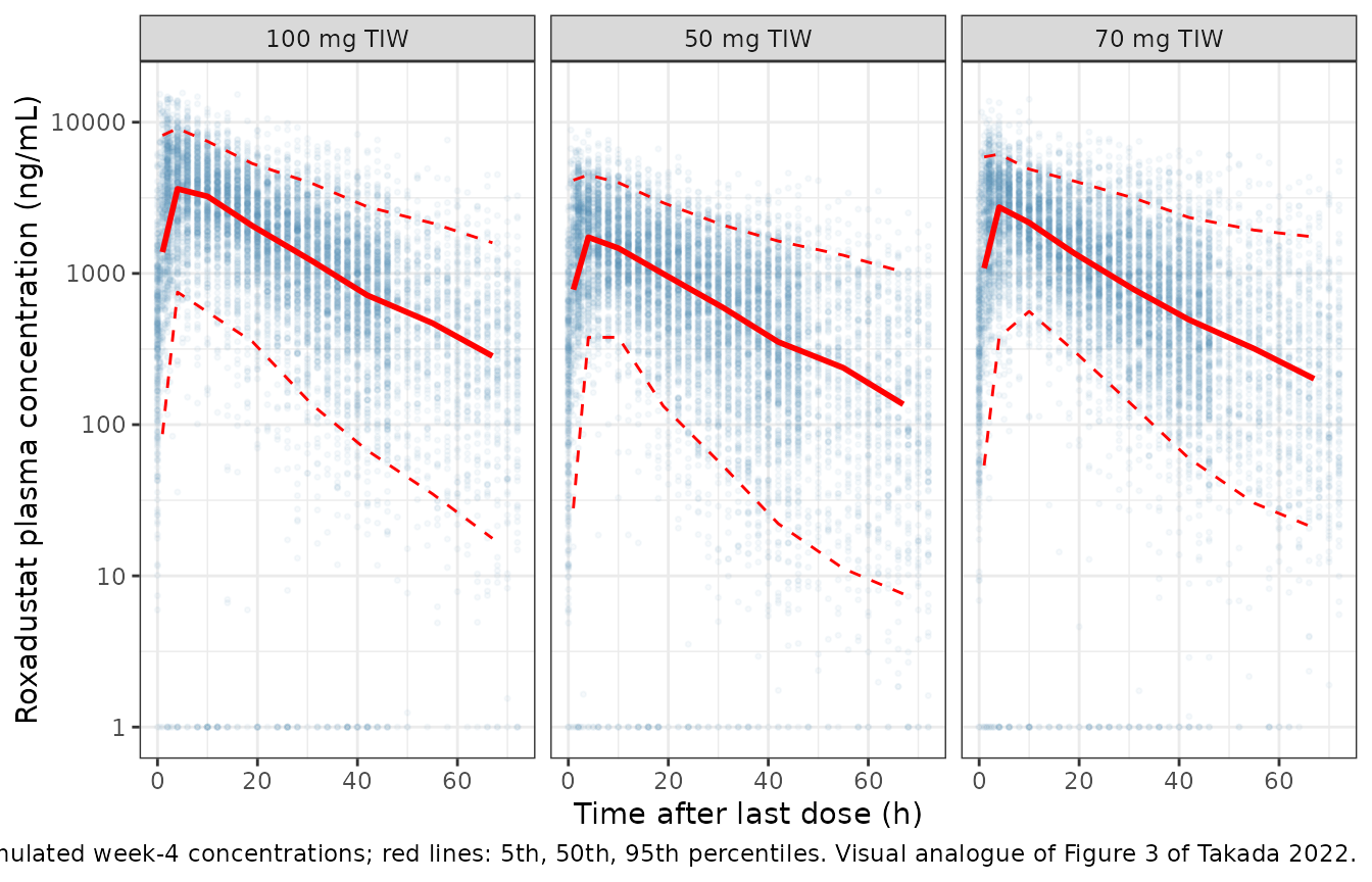
Steady-state NCA (PKNCA)
The paper publishes no NCA table, so the PKNCA block below
characterises the week-4 Monday-to-Wednesday dosing interval (504-552 h)
by arm. The structural checks are that exposure is dose proportional
(the model is linear) and that the median AUC over the 48-hour interval
matches the closed form F1 * Dose / (CL/F) for the cohort’s
own individual parameters, because with a 48-hour interval nearly the
whole dose is eliminated before the next one.
conc_ss <- sim |>
  dplyr::filter(time >= 504, time <= 552, !is.na(Cc)) |>
  dplyr::select(id, time, Cc, treatment)
dose_ss <- events |>
  dplyr::filter(evid == 1) |>
  dplyr::select(id, time, amt, treatment)

nca_ss <- PKNCA::pk.nca(PKNCA::PKNCAdata(
  PKNCA::PKNCAconc(conc_ss, Cc ~ time | treatment + id),
  PKNCA::PKNCAdose(dose_ss, amt ~ time | treatment + id),
  intervals = data.frame(
    start = 504, end = 552,
    cmax = TRUE, tmax = TRUE, auclast = TRUE, cmin = TRUE
  )
))

nca_tbl <- as.data.frame(nca_ss) |>
  dplyr::group_by(treatment, PPTESTCD) |>
  dplyr::summarise(median = signif(median(PPORRES, na.rm = TRUE), 3), .groups = "drop") |>
  tidyr::pivot_wider(names_from = PPTESTCD, values_from = median) |>
  dplyr::arrange(as.numeric(sub(" mg TIW", "", treatment)))

nca_tbl |>
  dplyr::rename(
    Arm = treatment,
    "Cmax (ng/mL)" = cmax,
    "Tmax (h)" = tmax,
    "AUC0-48 (ng*h/mL)" = auclast,
    "Cmin (ng/mL)" = cmin
  ) |>
knitr::kable(caption = "Median week-4 NCA over the 48-hour interval (504-552 h).")| Arm | AUC0-48 (ng*h/mL) | Cmax (ng/mL) | Cmin (ng/mL) | Tmax (h) |
|---|---|---|---|---|
| 50 mg TIW | 46100 | 2230 | 126 | 5.0 |
| 70 mg TIW | 60900 | 3190 | 188 | 4.0 |
| 100 mg TIW | 97400 | 4590 | 263 | 4.5 |
auc_by_id <- as.data.frame(nca_ss) |>
  dplyr::filter(PPTESTCD == "auclast") |>
  dplyr::select(id, treatment, auclast = PPORRES)
indiv <- sim |>
  dplyr::filter(time == 504) |>
  dplyr::distinct(id, cl, fdepot)
auc_chk <- auc_by_id |>
  dplyr::left_join(indiv, by = "id") |>
  dplyr::mutate(
    dose = as.numeric(sub(" mg TIW", "", treatment)),
    auc_closed = fdepot * dose / cl * 1000,
    pct_diff = 100 * (auclast / auc_closed - 1),
    auc_per_mg = auclast / dose
  )

auc_dn <- auc_chk |>
  dplyr::group_by(treatment) |>
  dplyr::summarise(median_auc_per_mg = median(auc_per_mg), .groups = "drop")
auc_dn
#> # A tibble: 3 × 2
#>   treatment  median_auc_per_mg
#>   <chr>                  <dbl>
#> 1 100 mg TIW              974.
#> 2 50 mg TIW               922.
#> 3 70 mg TIW               870.

stopifnot(
  # Centre of the interval-AUC vs closed-form distribution. A wrong unit,
  # dose or clearance would move this by tens of percent.
  # No tail-quantile gate: with a 184% CV on ka, roughly 8% of patients
  # absorb so slowly that much of a dose spills past the 48-hour interval.
  abs(median(auc_chk$pct_diff)) < 10,
  # Dose-normalised exposure is similar across arms (independent cohorts, so
  # only sampling noise separates them).
  max(auc_dn$median_auc_per_mg) / min(auc_dn$median_auc_per_mg) < 1.5
)
Assumptions and deviations
-
IIV scale. Table 4 labels IIV as %CV. The printed
confidence intervals are reproduced only when the percentage is
100 * sqrt(omega^2), so the model usesomega^2 = (CV/100)^2(0.1739, 0.0484, 3.389 for CL/F, Vc/F and ka). The very large ka variance (184% CV) is as published; the authors attribute it to the few absorption-phase samples. -
Residual error. Methods 2.4 defines
W = sqrt((IPRED * theta_prop)^2 + theta_add^2)withEPSfixed to variance 1, sopropSd = 0.439andaddSd = 1.88ng/mL are standard deviations, combined as in nlmixr2’s defaultprop() + add(). -
Phase II “no time separation” factor. Table 4 lists
a separate 0.935 factor on F1 for phosphate binders taken without time
separation in the phase II study; the Table 4 footnote calls it “the
additional effect of the phosphate binders due to the uncontrolled
intake”. The paper does not print the NONMEM code, so the model applies
the factor once, when
STUDY_PHASE2 = 1and at least one of the five binders is coadministered. This matches the single -6.5% AUCinf change in Figure 4. Whether the original code applied it once per binder (for patients taking several) is not stated. -
Multiple binders. The categorical model
theta1 * theta2^(0 or 1)is applied once per binder, so the F1 factors multiply when a patient takes more than one binder. The paper does not show a combination, but this follows from the Methods 2.5 equation. -
Age. Only the categorical age >= 65 years effect
is retained (a patient aged exactly 65 is in the >= 65 group). The
model takes continuous
AGEand applies the threshold internally. - Figure 4 age row. Figure 4 is labelled “Change of roxadustat AUCinf” but prints -20.8% for age >= 65 years, which is the change in CL/F. Results 3.4 states that AUCinf increases by 26.3%, which the model reproduces.
- Time-varying concomitant medications. The source built the binder indicators from daily administration records; the virtual cohort holds each patient’s binders constant for simplicity. The indicators may vary over time in a user’s data set.
- Table 3 versus text. The Results text gives 131 patients on lanthanum carbonate; Table 3 gives 139. The cohort uses the Table 3 phase III frequencies.
-
Screened, not retained. Sex, body weight, BMI,
serum albumin, AST, ALT, ALP, total protein, dialysis modality
(haemodialysis versus peritoneal dialysis), clopidogrel, dose, oral iron
and multivalent cation-containing drugs were tested and not retained
(Results 3.2-3.3). Covariates are recorded in the model’s
covariatesDataExcludedmetadata. - Errata. No erratum or correction was found for this article (Europe PMC and the journal landing page, checked 2026-10-02).