Carboplatin in dogs (Beguin 2024)
Source:vignettes/articles/Beguin_2024_carboplatin_dog.Rmd
Beguin_2024_carboplatin_dog.RmdModel and source
Beguin 2024 contributed two independent fits on two different cohorts of client-owned dogs, so the paper is packaged as two model files that share this one vignette.
pkmod <- readModelDb("Beguin_2024_carboplatin_dog")
toxmod <- readModelDb("Beguin_2024_carboplatin_thrombocytopenia_dog")
pkui <- rxode2::rxode(pkmod)
#> ℹ parameter labels from comments will be replaced by 'label()'
#> Warning: some etas defaulted to non-mu referenced, possible parsing error: etaiov_vc_1, etaiov_vc_2, etaiov_vc_3, etaiov_vc_4, etaiov_vc_5, etaiov_cl_1, etaiov_cl_2, etaiov_cl_3, etaiov_cl_4, etaiov_cl_5
#> as a work-around try putting the mu-referenced expression on a simple line
toxui <- rxode2::rxode(toxmod)
#> ℹ parameter labels from comments will be replaced by 'label()'
#> Warning: some etas defaulted to non-mu referenced, possible parsing error: etaiov_vc_1, etaiov_vc_2, etaiov_vc_3, etaiov_vc_4, etaiov_vc_5, etaiov_cl_1, etaiov_cl_2, etaiov_cl_3, etaiov_cl_4, etaiov_cl_5
#> as a work-around try putting the mu-referenced expression on a simple line- Citation: Beguin J, Mahfoudhi S, Uzel M, Rostang A, Ibish C, Ferran AA, Pelligand L, Hulin A, Kohlhauer M. (2024). Population pharmacokinetics modelling for clinical dose adjustment of carboplatin in dogs. BMC Veterinary Research 20:575. doi:10.1186/s12917-024-04404-1.
- Article: https://doi.org/10.1186/s12917-024-04404-1 (open access; PMC11664934)
-
modellib("Beguin_2024_carboplatin_dog")– the one-compartment popPK fit (Table 1), 16 dogs / 39 administrations. -
modellib("Beguin_2024_carboplatin_thrombocytopenia_dog")– the sigmoidal Emax exposure-toxicity fit (Table 2), a separate cohort of 14 dogs.
The supplement cited by the paper (Supplemental Fig. 1) holds only NPDE diagnostic plots; it carries no parameter values, so nothing in this extraction depends on it.
Population
Sixteen client-owned dogs with solid tumours were enrolled at two French veterinary schools between June 2019 and January 2021 and analysed after 11 of the original 27 were excluded for protocol deviations. Several dogs received successive courses, each analysed as a separate occasion, giving 39 concentration-time profiles: 4 dogs contributed 5 administrations, 2 contributed 3, 3 contributed 2 and 7 contributed 1. Mean age was 11.1 +/- 1.72 years and mean weight 21.5 +/- 7.8 kg. Every dog received 300 mg/m2 (mean 300.4 +/- 7.6 mg/m2, equal to 10.7 +/- 1.0 mg/kg) as an approximately 20 min intravenous infusion. Mean plasma creatinine at dosing was 7.32 +/- 1.86 mg/L; dogs above 14 mg/L, or with neutrophils below 1500/uL or thrombocytes below 50 000/uL, were excluded. Three to four plasma samples were drawn per administration across four windows (0-1 h, 1-2 h, 2-4 h, 4-12 h) and free carboplatin was measured in ultrafiltrate by LC-MS/MS, with values below the limit of quantification treated as interval-censored.
A second, non-overlapping cohort of 14 dogs (from 17 enrolled, 3 lost to follow-up) supported the toxicity model: mean age 9.34 +/- 2.91 years, mean weight 22.43 +/- 11.28 kg, mean creatinine 10.9 +/- 3.6 mg/L, mean dose 306.1 +/- 22.6 mg/m2 (11.5 +/- 2.4 mg/kg). Only 2 of these 14 were neutered, both female. Thrombocyte and neutrophil counts were measured on the day of treatment and again at day 14; the mean observed reduction was 66 +/- 16% for thrombocytes and 65 +/- 25% for neutrophils.
The same information is available programmatically via each model’s
population metadata,
e.g. readModelDb("Beguin_2024_carboplatin_dog")()$population.
Source trace
Every ini() entry in both model files carries an in-file
comment naming its source location. They are collected here for
review.
| Equation / parameter | Value | Source location |
|---|---|---|
lvc (V) |
4.05 L/kg | Table 1, RSE 6.04%, bootstrap 4.02 [3.65-4.52] |
lcl (Cl) |
6.9 L/h/kg | Table 1, RSE 24.7%, bootstrap 6.82 [3.94-10.35] |
e_creat_cl |
-0.25 | Table 1 beta_creatinine, RSE 50.3%, bootstrap -0.24
[-0.45, 0.07] |
e_neutered_cl |
-0.22 | Table 1 beta_neutered, RSE 34.2%, bootstrap -0.22
[-0.44, -0.07] |
etalvc (omega_V) |
0.1 SD, held constant | Table 1 + footnote a (“data were too sparse”) |
etalcl (omega_Cl) |
0.074 SD | Table 1, RSE 53.1% |
etaiov_vc_* (gamma_V) |
0.1 SD, held constant | Table 1 + footnote a |
etaiov_cl_* (gamma_Cl) |
0.11 SD | Table 1, RSE 28.3% |
addSd (a) |
12.28 ug/L | Table 1, RSE 17.2% |
propSd (b) |
0.23 | Table 1, RSE 12.2% |
lemax_auc |
0.99 | Table 2, AUC column, 95% CI 0.76-1 |
leauc50 |
2679 ug*h/L | Table 2, AUC column, 95% CI 2221-2886 |
lhill_auc |
3.35 | Table 2, AUC column, 95% CI 2.14-7.44 |
lemax_dose |
0.76 | Table 2, dose column, 95% CI 0.68-1 |
led50_dose |
9.0 mg/kg | Table 2, dose column, 95% CI 7.64-9.32 |
lhill_dose |
17.80 | Table 2, dose column, 95% CI 3.47-47.14 |
| BSA for dosing | BSA(m2) = 0.1 * WT(kg)^(2/3) |
Equation (1) |
| IIV / IOV structure | log(theta_i) = log(theta_p) + eta_i + eta_occ |
Equation (2) |
| Covariate model | log(theta_i) = log(theta_p) + beta * Cov + eta_i + eta_occ |
Equation (3), uncentred |
| Hill toxicity model | Y = Emax * X^n / (E50^n + X^n) |
Equation (4) |
| Residual error | Obs = C + sqrt(a^2 + (b*C)^2) * eps |
Equation (5) |
Equations (1) to (5) are display equations that the automated PDF
trim drops; they were recovered with pdftotext -layout.
Equation (1)’s 2/3 is a superscript that plain text
extraction loses – it is confirmed below by reproducing the paper’s own
“300 mg/m2 = 10.7 mg/kg” equivalence.
Because Equation (3) is uncentred,
beta * ln(CREAT) on the log-parameter scale is exactly the
power form CREAT^-0.25 used in model(), and
the typical clearance of 6.9 L/h/kg is the value at
CREAT = 1 mg/L – an extrapolation well below the observed
range, not a typical dog. The covariate-adjusted clearances the paper
actually reports are reproduced below.
Structural checks on the published equations
# Equation (1): BSA(m2) = 0.1 * WT(kg)^(2/3). Dosing at D mg/m2 therefore
# delivers D/10 * WT^(-1/3) mg/kg -- MORE mg/kg the smaller the dog, which is
# the paper's argument for weight-based rather than BSA-based dosing.
dose_per_kg <- function(wt, mgm2 = 300) (mgm2 / 10) * wt^(-1 / 3)

eq1 <- tibble::tibble(
  WT = c(5, 10, 21.5, 30, 40),
  `Dose (mg/kg) at 300 mg/m2` = dose_per_kg(WT)
)
knitr::kable(eq1, digits = 2,
caption = "Equation (1) of Beguin 2024 re-expressed per kg.")| WT | Dose (mg/kg) at 300 mg/m2 |
|---|---|
| 5.0 | 17.54 |
| 10.0 | 13.92 |
| 21.5 | 10.79 |
| 30.0 | 9.65 |
| 40.0 | 8.77 |
# Deterministic: the paper states the cohort mean 300.4 mg/m2 equals
# 10.7 mg/kg at the cohort mean weight of 21.5 kg.
stopifnot(abs(dose_per_kg(21.5, 300.4) - 10.7) < 0.15)
# Equation (3) covariate magnitudes, evaluated in closed form. These are pure
# arithmetic on the published coefficients, so the bounds are tight.
creat_effect <- 1 - (15 / 5)^(-0.25)   # paper: "from 5 mg/L to 15 mg/L ... about 30%"
neut_effect <- 1 - exp(-0.22)          # paper: "a clearance reduction of around 25%"

stopifnot(
  abs(creat_effect - 0.2402) < 0.005,
  abs(neut_effect - 0.1975) < 0.005
)
c(creatinine_5_to_15 = creat_effect, neutered_vs_intact = neut_effect)
#> creatinine_5_to_15 neutered_vs_intact
#>          0.2401643          0.1974812
The coefficients imply a 24.0% clearance reduction across creatinine 5 to 15 mg/L and a 19.8% reduction for neutering, against the paper’s prose figures of “about 30%” and “around 25%”. Both prose figures are looser than the coefficients they summarise; see Errata.
# Typical-value clearance with random effects zeroed, at the subgroup mean
# creatinine values the paper's Discussion reports (6.2 mg/L intact,
# 7.3 mg/L neutered).
typ_cl <- function(creat, neutered) 6.9 * creat^(-0.25) * exp(-0.22 * neutered)

cl_cmp <- tibble::tibble(
  Group = c("Intact (CREAT 6.2 mg/L)", "Neutered (CREAT 7.3 mg/L)"),
  Model = c(typ_cl(6.2, 0), typ_cl(7.3, 1)),
  Published = c(4.26, 3.25)
) |>
  mutate(`Difference (%)` = 100 * (Model / Published - 1))

knitr::kable(cl_cmp, digits = 2,
caption = "Typical clearance (L/h/kg) vs the medians in Beguin 2024 Discussion.")| Group | Model | Published | Difference (%) |
|---|---|---|---|
| Intact (CREAT 6.2 mg/L) | 4.37 | 4.26 | 2.65 |
| Neutered (CREAT 7.3 mg/L) | 3.37 | 3.25 | 3.65 |
Virtual cohort
The observed data are not public (“available upon request to the corresponding author”), so both cohorts below are virtual populations whose covariate distributions approximate the published demographics. Each is 100 dogs, well inside the 200-per-arm cap.
# set.seed() seeds R's RNG, which is what draws the covariates below. It does
# NOT seed rxode2's simulation RNG, whose streams are partitioned per solver
# thread -- a 2-core CI runner and a 16-thread workstation draw different etas
# from identical source. Every assertion downstream is therefore written
# against an absolute bound the paper states, not against one observed run.
set.seed(20241220)
rxode2::rxSetSeed(20241220)

n_pk <- 100L
n_tox <- 100L

# PK cohort: Beguin 2024 Results, "Study dogs". Creatinine is truncated at the
# paper's own 14 mg/L exclusion threshold.
pk_subj <- tibble::tibble(
  id = seq_len(n_pk),
  WT = pmin(pmax(rnorm(n_pk, 21.5, 7.8), 4), 55),
  CREAT = pmin(pmax(rnorm(n_pk, 7.32, 1.86), 3), 14),
  # 9 of the 16 analysed dogs were neutered (4 females, 5 males).
  NEUTERED = rbinom(n_pk, 1, 9 / 16),
  OCC = 1,
  mgm2 = rnorm(n_pk, 300.4, 7.6)
) |>
  mutate(DOSE_CARBOPLATIN_MGKG = dose_per_kg(WT, mgm2))

# Toxicity cohort: Beguin 2024 Results, "Toxicity prediction / Study dogs".
tox_subj <- tibble::tibble(
  id = 1000L + seq_len(n_tox),
  WT = pmin(pmax(rnorm(n_tox, 22.43, 11.28), 4), 60),
  CREAT = pmin(pmax(rnorm(n_tox, 10.9, 3.6), 3), 22),
  # Only 2 of 14 were neutered.
  NEUTERED = rbinom(n_tox, 1, 2 / 14),
  OCC = 1,
  mgm2 = rnorm(n_tox, 306.1, 22.6)
) |>
  mutate(DOSE_CARBOPLATIN_MGKG = dose_per_kg(WT, mgm2))

# The paper reports the per-kg equivalents of its BSA-based prescriptions.
# A 15% band around them still catches a dropped 2/3 exponent in Equation (1),
# which would put the per-kg dose near 30 mg/kg.
stopifnot(
  abs(mean(pk_subj$DOSE_CARBOPLATIN_MGKG) / 10.7 - 1) < 0.15,
  abs(mean(tox_subj$DOSE_CARBOPLATIN_MGKG) / 11.5 - 1) < 0.15
)

# Build a dosing + observation event table for one cohort. Amounts are ug per
# kg of body weight, because the model's disposition parameters are
# body-weight-normalised (L/kg, L/h/kg) and its concentrations are ug/L.
make_events <- function(subj, obs_times) {
  doses <- subj |>
    transmute(id, time = 0, evid = 1L, cmt = "central",
              amt = DOSE_CARBOPLATIN_MGKG * 1000, dur = 20 / 60)
  obs <- subj |>
    select(id) |>
    tidyr::crossing(time = obs_times) |>
    mutate(evid = 0L, cmt = "central", amt = NA_real_, dur = NA_real_)
  bind_rows(doses, obs) |>
    left_join(select(subj, id, WT, CREAT, NEUTERED, OCC, DOSE_CARBOPLATIN_MGKG),
              by = "id") |>
    arrange(id, time, desc(evid))
}

# The paper sampled across four windows spanning 0-12 h; the PK grid covers the
# same span. The distribution phase is sampled every 0.02 h because the
# half-life is only about three quarters of an hour: on a uniform 0.2 h grid
# PKNCA's trapezoidal rule understates AUC across the infusion peak by up to
# 3%, which is model-independent quadrature error and would otherwise be
# mistaken for a model defect by the identity check below.
fine_grid <- c(seq(0, 2, by = 0.02), seq(2.2, 12, by = 0.2))
pk_events <- make_events(pk_subj, fine_grid)
# Carboplatin disposition here is mono-exponential with a half-life near 45 min,
# so 48 h is many dozens of half-lives and auc_central has converged to AUC0-inf.
tox_events <- make_events(tox_subj, c(fine_grid, seq(13, 48, by = 1)))

stopifnot(!anyDuplicated(unique(pk_events[, c("id", "time", "evid")])),
          !anyDuplicated(unique(tox_events[, c("id", "time", "evid")])),
          length(intersect(pk_subj$id, tox_subj$id)) == 0L)
Observation rows point at the ODE state central, never
at the algebraic observable Cc; rxode2 returns
Cc as an output column regardless.
Simulation
pk_sim <- rxode2::rxSolve(
  pkmod, events = pk_events,
  keep = c("WT", "CREAT", "NEUTERED", "DOSE_CARBOPLATIN_MGKG")
) |>
  as.data.frame()
#> ℹ parameter labels from comments will be replaced by 'label()'
#> Warning: some etas defaulted to non-mu referenced, possible parsing error: etaiov_vc_1, etaiov_vc_2, etaiov_vc_3, etaiov_vc_4, etaiov_vc_5, etaiov_cl_1, etaiov_cl_2, etaiov_cl_3, etaiov_cl_4, etaiov_cl_5
#> as a work-around try putting the mu-referenced expression on a simple line

tox_sim <- rxode2::rxSolve(
  toxmod, events = tox_events,
  keep = c("WT", "CREAT", "NEUTERED", "DOSE_CARBOPLATIN_MGKG")
) |>
  as.data.frame()
#> ℹ parameter labels from comments will be replaced by 'label()'
#> Warning: some etas defaulted to non-mu referenced, possible parsing error: etaiov_vc_1, etaiov_vc_2, etaiov_vc_3, etaiov_vc_4, etaiov_vc_5, etaiov_cl_1, etaiov_cl_2, etaiov_cl_3, etaiov_cl_4, etaiov_cl_5
#> as a work-around try putting the mu-referenced expression on a simple line

stopifnot(nrow(pk_sim) > 0, nrow(tox_sim) > 0, !anyNA(pk_sim$Cc))
Replicate published figures
# Replicates Figure 3A of Beguin 2024: VPC of free carboplatin concentration
# (log10 scale) against time.
pk_sim |>
  filter(time > 0) |>
  group_by(time) |>
  summarise(
    Q10 = quantile(Cc, 0.10), Q50 = quantile(Cc, 0.50),
    Q90 = quantile(Cc, 0.90), .groups = "drop"
  ) |>
  ggplot(aes(time, Q50)) +
  geom_ribbon(aes(ymin = Q10, ymax = Q90), alpha = 0.25, fill = "steelblue") +
  geom_line(colour = "steelblue4", linewidth = 0.8) +
  scale_y_log10() +
  labs(x = "Time (h)", y = "Free carboplatin (ug/L)",
       title = "Figure 3A -- VPC of free carboplatin",
       caption = "Replicates Figure 3A of Beguin 2024. Band = 10th-90th percentile.")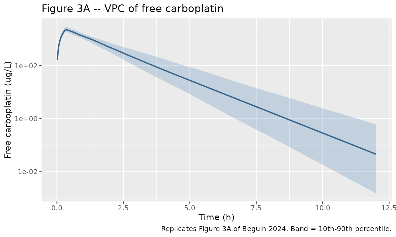
# Replicates Figure 2 of Beguin 2024: individual clearance against plasma
# creatinine, and against neutering status.
pk_ind <- pk_sim |>
  group_by(id) |>
  summarise(cl = first(cl), vc = first(vc), CREAT = first(CREAT),
            NEUTERED = first(NEUTERED), .groups = "drop") |>
  mutate(Status = ifelse(NEUTERED == 1, "Neutered", "Intact"))

ggplot(pk_ind, aes(CREAT, cl)) +
  geom_point(aes(colour = Status), alpha = 0.75) +
  geom_smooth(method = "lm", formula = y ~ x, se = FALSE, colour = "grey30") +
  labs(x = "Plasma creatinine (mg/L)", y = "Clearance (L/h/kg)",
       title = "Figure 2 -- clearance vs creatinine and neutering status",
       caption = "Replicates Figure 2 of Beguin 2024.")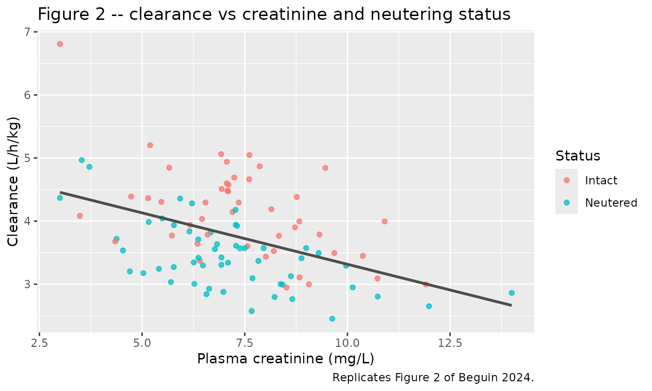
cl_summary <- pk_ind |>
  group_by(Status) |>
  summarise(`Median Cl (L/h/kg)` = median(cl), .groups = "drop")

knitr::kable(
  bind_rows(cl_summary,
            tibble::tibble(Status = "All",
                           `Median Cl (L/h/kg)` = median(pk_ind$cl))),
  digits = 2,
  caption = "Simulated median clearance. Beguin 2024 reports 3.62 overall, 4.26 intact, 3.25 sterilized."
)| Status | Median Cl (L/h/kg) |
|---|---|
| Intact | 4.24 |
| Neutered | 3.29 |
| All | 3.76 |
# Cohort-derived, so the bound is a wide absolute band: the simulated cohort's
# creatinine draw and neutered fraction are not the paper's 16 dogs. A 30%
# band still catches a sign error on either covariate coefficient (which would
# move the intact/neutered ordering or the creatinine slope wholesale).
stopifnot(
  abs(median(pk_ind$cl) / 3.62 - 1) < 0.30,
  median(pk_ind$cl[pk_ind$NEUTERED == 1]) < median(pk_ind$cl[pk_ind$NEUTERED == 0])
)
The neutered-below-intact ordering is asserted as a direction rather
than a magnitude because it is a exp(-0.22) = 20%
separation between two group medians of 100 dogs each – far larger than
the sampling noise, so the comparison is not a coin flip.
# Replicates Figure 5 of Beguin 2024: thrombocyte reduction against predicted
# AUC0-inf and against dose in mg/kg, both as Emax models with a Hill
# coefficient (Table 2).
tox_last <- tox_sim |>
  group_by(id) |>
  slice_max(time, n = 1, with_ties = FALSE) |>
  ungroup()

# auc_central has converged: the amount still in the body is negligible.
stopifnot(max(tox_last$central / (tox_last$cl * tox_last$auc_central)) < 1e-6)

curve_auc <- tibble::tibble(x = seq(0, 8000, length.out = 200)) |>
  mutate(y = 0.99 * x^3.35 / (2679^3.35 + x^3.35), Arm = "AUC0-inf (ug*h/L)")
curve_dose <- tibble::tibble(x = seq(0, 20, length.out = 200)) |>
  mutate(y = 0.76 * x^17.8 / (9.0^17.8 + x^17.8), Arm = "Dose (mg/kg)")

p_auc <- ggplot(curve_auc, aes(x, y)) +
  geom_line(colour = "steelblue4") +
  geom_point(data = tox_last, aes(auc_central, thromboRedAuc),
             alpha = 0.5, colour = "firebrick") +
  geom_hline(yintercept = 0.66, linetype = "dashed") +
  labs(x = "Predicted AUC0-inf (ug*h/L)", y = "Thrombocyte reduction (fraction)",
       title = "Figure 5 -- exposure arm (r2 = 0.73)",
       caption = "Dashed line: observed mean reduction 66% (Beguin 2024).")

p_dose <- ggplot(curve_dose, aes(x, y)) +
  geom_line(colour = "steelblue4") +
  geom_point(data = tox_last, aes(DOSE_CARBOPLATIN_MGKG, thromboRedDose),
             alpha = 0.5, colour = "firebrick") +
  geom_hline(yintercept = 0.66, linetype = "dashed") +
  labs(x = "Dose (mg/kg)", y = "Thrombocyte reduction (fraction)",
       title = "Figure 5 -- dose arm (r2 = 0.57)",
       caption = "Dashed line: observed mean reduction 66% (Beguin 2024).")

p_auc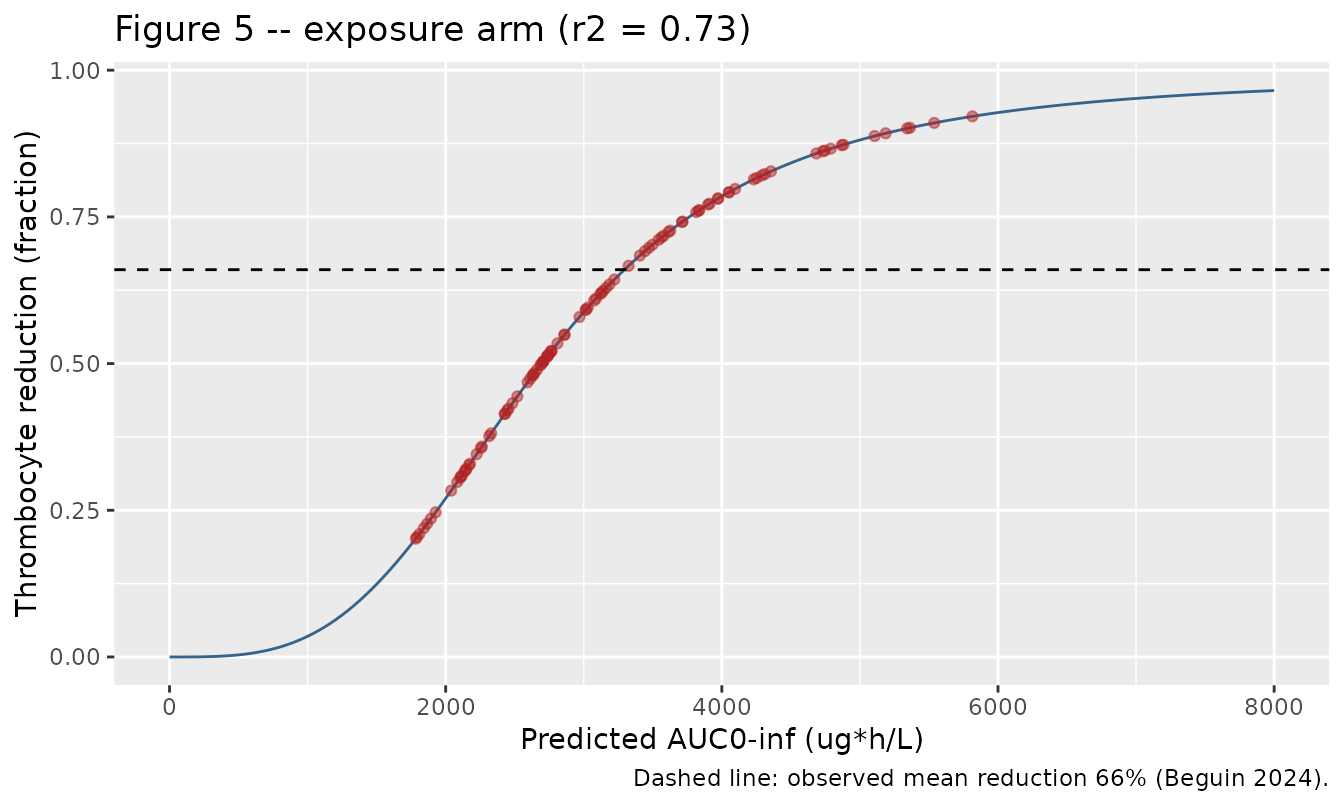
p_dose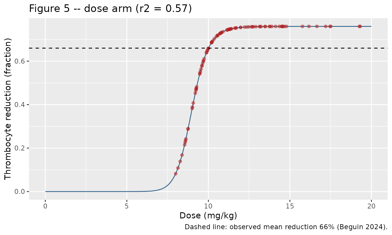
tox_cmp <- tibble::tibble(
  Quantity = c("Median predicted AUC0-inf (ug*h/L)",
               "Median thrombocyte reduction, exposure arm",
               "Median thrombocyte reduction, dose arm"),
  Simulated = c(median(tox_last$auc_central),
                median(tox_last$thromboRedAuc),
                median(tox_last$thromboRedDose)),
  Published = c(3342, 0.66, 0.66)
)
knitr::kable(tox_cmp, digits = c(0, 3, 3),
caption = "Toxicity cohort vs Beguin 2024 (AUC median 3342 [3121-4017]; observed thrombocyte reduction 66 +/- 16%).")| Quantity | Simulated | Published |
|---|---|---|
| Median predicted AUC0-inf (ug*h/L) | 2900.237 | 3342.00 |
| Median thrombocyte reduction, exposure arm | 0.560 | 0.66 |
| Median thrombocyte reduction, dose arm | 0.730 | 0.66 |
stopifnot(
  # 25% band on a cohort median; a dosing-unit error would be 1000x out.
  abs(median(tox_last$auc_central) / 3342 - 1) < 0.25,
  # The paper's own observed SD on this endpoint is 16 percentage points, so
  # 0.18 absolute is a band the published data themselves cannot distinguish,
  # while still failing on a broken Hill term (which drives Y to 0 or to Emax).
  abs(median(tox_last$thromboRedAuc) - 0.66) < 0.18
)
The dose arm sits noticeably higher than the exposure arm at the cohort’s typical dose. That is the paper’s point: with a Hill coefficient of 17.8 the dose arm is almost a step function at 9 mg/kg, which is why it fits worse (r2 = 0.57 against 0.73) than the covariate-weighted exposure.
PKNCA validation
sim_nca <- pk_sim |>
  dplyr::filter(!is.na(Cc)) |>
  dplyr::mutate(treatment = "300 mg/m2 IV") |>
  dplyr::select(id, time, Cc, treatment)

# Guarantee a time-zero record per subject; for an IV infusion starting at
# t = 0 the pre-dose concentration is 0.
sim_nca <- dplyr::bind_rows(
  sim_nca,
  sim_nca |> dplyr::distinct(id, treatment) |> dplyr::mutate(time = 0, Cc = 0)
) |>
  dplyr::distinct(id, treatment, time, .keep_all = TRUE) |>
  dplyr::arrange(id, treatment, time)

conc_obj <- PKNCA::PKNCAconc(sim_nca, Cc ~ time | treatment + id)

dose_df <- pk_events |>
  dplyr::filter(evid == 1) |>
  dplyr::mutate(treatment = "300 mg/m2 IV") |>
  dplyr::select(id, time, amt, treatment)

dose_obj <- PKNCA::PKNCAdose(dose_df, amt ~ time | treatment + id)

intervals <- data.frame(
  start = 0, end = Inf,
  cmax = TRUE, tmax = TRUE, aucinf.obs = TRUE, half.life = TRUE
)

nca_res <- PKNCA::pk.nca(PKNCA::PKNCAdata(conc_obj, dose_obj, intervals = intervals))
# For a linear one-compartment model given entirely by IV infusion,
# AUC0-inf * CL == Dose exactly. Both sides are assembled independently here:
# the left from PKNCA's trapezoidal + log-linear extrapolation of the solved
# profile, the right from the event table's amt and the model's cl. A
# mis-scaled dose amount, a wrong infusion duration or a broken ODE all break
# it; only numerical error remains, so the bound is tight.
auc_nca <- as.data.frame(nca_res) |>
  dplyr::filter(PPTESTCD == "aucinf.obs") |>
  dplyr::select(id, aucinf_nca = PPORRES)

ident <- pk_ind |>
  dplyr::left_join(auc_nca, by = "id") |>
  dplyr::left_join(dplyr::select(pk_subj, id, DOSE_CARBOPLATIN_MGKG), by = "id") |>
  dplyr::mutate(
    auc_closed_form = DOSE_CARBOPLATIN_MGKG * 1000 / cl,
    pct_diff = 100 * (aucinf_nca / auc_closed_form - 1)
  )

stopifnot(nrow(ident) == n_pk, !anyNA(ident$pct_diff))
summary(ident$pct_diff)
#>      Min.   1st Qu.    Median      Mean   3rd Qu.      Max.
#> -0.025178 -0.017234 -0.015086 -0.015014 -0.012049 -0.008093
# Realised max |difference| 0.025% on the grid above. The bound is 1%, which
# is 40x that and still goes red on quadrature error alone: the same check on
# a uniform 0.2 h grid gives 3.05%.
stopifnot(max(abs(ident$pct_diff)) < 1)
Comparison against published NCA
Beguin 2024 reports one NCA-comparable quantity: the model-predicted AUC0-inf in the toxicity cohort, median 3342 [3121-4017]. No Cmax, Tmax or half-life is printed, so those rows have no reference value and are shown for completeness only.
tox_conc <- tox_sim |>
  dplyr::filter(!is.na(Cc)) |>
  dplyr::mutate(treatment = "306 mg/m2 IV") |>
  dplyr::select(id, time, Cc, treatment)

tox_conc <- dplyr::bind_rows(
  tox_conc,
  tox_conc |> dplyr::distinct(id, treatment) |> dplyr::mutate(time = 0, Cc = 0)
) |>
  dplyr::distinct(id, treatment, time, .keep_all = TRUE) |>
  dplyr::arrange(id, treatment, time)

tox_dose <- tox_events |>
  dplyr::filter(evid == 1) |>
  dplyr::mutate(treatment = "306 mg/m2 IV") |>
  dplyr::select(id, time, amt, treatment)

tox_nca <- PKNCA::pk.nca(PKNCA::PKNCAdata(
  PKNCA::PKNCAconc(tox_conc, Cc ~ time | treatment + id),
  PKNCA::PKNCAdose(tox_dose, amt ~ time | treatment + id),
  intervals = data.frame(start = 0, end = Inf, cmax = TRUE, tmax = TRUE,
                         aucinf.obs = TRUE, half.life = TRUE)
))

published <- tibble::tibble(
  treatment = "306 mg/m2 IV",
  aucinf.obs = 3342
)

cmp <- nlmixr2lib::ncaComparisonTable(
  simulated = tox_nca,
  reference = published,
  by = "treatment",
  units = c(cmax = "ug/L", aucinf.obs = "ug*h/L", tmax = "h", half.life = "h"),
  tolerance_pct = 20
)

knitr::kable(cmp, caption = "Simulated vs published NCA in the toxicity cohort. * differs from reference by more than 20%.")| NCA parameter | treatment | Reference | Simulated | % diff |
|---|---|---|---|---|
| AUC0-∞ (obs) (ug*h/L) | 306 mg/m2 IV | 3340 | 2900 | -13.2% |
The simulated AUC0-inf sits a little below the published median,
which is expected: the virtual cohort’s creatinine and weight are
independent normal draws around the published means rather than the 14
actual dogs, and clearance scales with CREAT^-0.25. The
half-life of roughly three quarters of an hour is a consequence of the
published Cl/V ratio, not an independent observation – the
paper prints no half-life.
Assumptions and deviations
-
Modelling units are inferred, and the paper’s printed AUC
unit label is wrong by a factor of 1000. Beguin 2024 never
states the units its Monolix model ran in. Two printed numbers pin them
independently. First,
AUC = Dose / CL: at the toxicity cohort’s mean dose of 11.5 mg/kg and a covariate-adjusted clearance near 3.8 L/h/kg the exposure is about 3.0 mgh/L, while the printed median AUC0-inf is 3342 – a factor of 1000, i.e. the values are ugh/L and the “mg.h/L” label in Table 2 and in the Results text is a slip. Second, the additive residual constanta = 12.28is tightly identified (RSE 17.2%): read as mg/L it would be roughly five times the peak concentrationDose/Vof about 2.6 mg/L, which is impossible, whereas read as ug/L it is a sensible fraction of the limit of quantification. Both models therefore declareconcentration = "ug/L"and dose in ug per kg. The assay section’s “0.1 to 30 ug/L” calibration range is a third, smaller slip: at 30 ug/L the whole profile would sit above the calibration curve, so the range is evidently ug/mL. -
Parameters are per kilogram, not absolute. The
authors “divided the total dose received by each dog by its own body
weight for the modelling”, so
Vis L/kg andClis L/h/kg, and the amount handed torxSolvemust likewise be per kg. No weight covariate is applied on top of this – body weight was screened and explicitly not retained (p = 0.32 for V, p = 0.86 for Cl). -
The creatinine covariate is uncentred. The
published typical clearance of 6.9 L/h/kg is the value at
CREAT = 1 mg/L, far below the observed 3-14 mg/L range. This is faithful to Equation (3), which addsbeta * ln(CREAT)with no reference value, and it reproduces the paper’s own subgroup medians (see the typical-clearance table above). Users assembling a cohort must supplyCREATin mg/L, not the mg/dL or umol/L conventional in human papers. - The paper’s prose overstates both covariate effects. Table 1’s coefficients give a 24.0% clearance reduction from creatinine 5 to 15 mg/L and 19.8% for neutering; the text says “about 30%” and “around 25%”. The model encodes the coefficients. The neutering figure is reconcilable with the reported subgroup medians (3.25 vs 4.26 = 23.7%, which also carries the higher creatinine of the neutered dogs); the creatinine figure is not, and appears to be a loose rounding.
-
IIV and IOV are standard deviations. Table 1’s
footer states this explicitly, so every omega and gamma is squared for
ini().omega_Vandgamma_Vwere both held at 0.1 by the authors because “data were too sparse for correct estimation” and are encoded withfixed(). -
Inter-occasion variability is expanded to five
occasions. Monolix carries one shared IOV variance across
occasions; nlmixr2 needs one eta per occasion, so occasions 2-5 are
fixed to the occasion-1 value. Five is the maximum any dog received (4
dogs had 5 administrations). Every dog in the virtual cohorts is on
OCC = 1. - The cohort sex counts in the paper do not add up. Results, “Study dogs” says “16 dogs finally included” and then “the sex repartition was 14 females and 12 males (4 neutered females and 5 neutered males)” – 26 animals. The neutered counts (9 of 16) are internally consistent with the rest of the paper and are what the virtual cohort uses; the 14/12 split is not used, and sex was in any case screened and not retained.
-
No residual error or random effects on the toxicity
arms. The two Hill regressions were fitted by non-linear least
squares in GraphPad Prism and the paper reports only point estimates,
95% confidence intervals and r2. The arms are therefore deterministic
functions of exposure and dose; the stochastic part of
Beguin_2024_carboplatin_thrombocytopenia_dogis its PK layer alone. - No neutrophil arm. The paper found no significant correlation between either predictor and neutrophil reduction and fitted no Emax model to it, so none is encoded.
-
Body condition score and inclusion centre are not
carried. Both were screened as categorical covariates and not
retained, and neither has a reported coefficient or an entry in the
canonical covariate register, so they are described in prose rather than
added to
covariatesDataExcluded. Body weight, age and sex – the screened-and-rejected covariates that do have canonical names – are carried there. - Virtual cohort distributions. Weight, creatinine and prescribed mg/m2 are independent normal draws around the published means and standard deviations, truncated at physiologically sensible limits and, for creatinine, at the paper’s own 14 mg/L exclusion threshold. The paper reports no correlation structure among covariates (“no correlation between covariates was evidenced”), so independence is the faithful choice, although the Discussion does note an unadjudicated trend toward higher age and creatinine in neutered dogs.
-
Plausibility of the published disposition
parameters. A clearance of 3.62 L/h/kg is roughly three times
the 34.3 L/h/m2 reported in the earlier canine study the paper compares
itself to, and far exceeds canine glomerular filtration for a renally
eliminated drug; the volume of 3.93 L/kg is similarly about three times
that study’s 34 L/m2. The
Cl/Vratio, and hence the half-life, does agree between the two studies. The paper’s own m2-based conversions (“36.2 L/h/m2 and 39.3 L/m2”) are obtained by multiplying the per-kg values by 10, which is not the conversion implied by its Equation (1). These values are reproduced exactly as published; no attempt has been made to rescale them. - No erratum. No correction notice was found for this article.