Dasatinib (Hassouneh 2024)

Model and source

mod <- rxode2::rxode2(readModelDb("Hassouneh_2024_dasatinib"))
#> ℹ parameter labels from comments will be replaced by 'label()'
#> Warning: some etas defaulted to non-mu referenced, possible parsing error: etaiov_ktr_1, etaiov_ktr_2, etaiov_mtt_1, etaiov_mtt_2, etaiov_ka_1, etaiov_ka_2, etaiov_cl_1, etaiov_cl_2
#> as a work-around try putting the mu-referenced expression on a simple line

Citation: Hassouneh WB, Al-Ghazawi MA, Saleh MI, Najib N. Population Pharmacokinetics of Dasatinib in Healthy Subjects. Pharmaceuticals (Basel). 2024 May 23;17(6):671. doi:10.3390/ph17060671.
Article: https://doi.org/10.3390/ph17060671
PubMed Central: https://www.ncbi.nlm.nih.gov/pmc/articles/PMC11206811/

Hassouneh 2024 asks why dasatinib is so variable. The answer the paper reaches is body mass index acting on the absorption rate constant: of roughly twenty screened demographics, laboratory values and concomitant medications, BMI on Ka was the only covariate that survived COSSAC forward inclusion and backward elimination. The structural model is a two-compartment disposition model fed by a Savic transit-compartment chain, with interindividual and interoccasion variability on the two absorption-chain parameters, on Ka, and on CL.

This vignette does three things: it reproduces the paper’s own visual predictive check from the packaged parameters, it establishes closed-form identity gates on the transit chain and the AUC, and it documents (with a numeric falsification) the one place where the published covariate equation cannot be taken literally.

Population

110 healthy Middle Eastern male volunteers, out of 116 enrolled, contributed 4180 plasma dasatinib concentrations - exactly 110 subjects x 2 SPRYCEL dosing occasions x 19 samples. The data come from the two reference-product periods of a four-period full-replicate bioequivalence study run at the International Pharmaceutical Research Center in Amman, Jordan; each occasion administered a single 140 mg SPRYCEL film-coated tablet under fasting conditions with 240 mL of water, with no food for 4 h post-dose. Before analysis the dataset was split: 88 subjects estimated the model and 22 (20%) were held out for internal validation.

Baseline characteristics (Table 2): median age 33 years [18-49] (mean 32 +/- 8.36), median weight 70 kg [51-100] (mean 72 +/- 12.71), median height 175 cm [160-192], median BMI 22.9 kg/m^2 [18.6-29.8] (mean 23.6 +/- 3.50). 85.34% were smokers. Eligibility required age 18-55 years and BMI 18.5-30.0 kg/m^2, so the cohort is healthy, male, Middle Eastern, and spans only the normal-to-overweight BMI band; the Discussion notes about 35% of subjects were overweight or obese (BMI > 25 kg/m^2). The Conclusions list the healthy-volunteer composition, the resulting compression of every laboratory covariate into its reference range, and the single-sex single-ethnicity cohort as the study’s limitations.

The same information is available programmatically via readModelDb("Hassouneh_2024_dasatinib")()$population.

Source trace

Every ini() entry carries an in-file comment naming its source location in Hassouneh 2024. The table collects them in one place.

Model element	Value as encoded	Source location
`lktr` (Ktr)	18.8 1/h	Table 3, row “Ktr” (RSE 9.34%)
`lmtt` (Mtt)	0.48 h	Table 3, row “Mtt” (RSE 4.63%)
`lka` (Ka)	0.37 1/h at BMI 22.9	Table 3, row “Ka” (RSE 4.8%); covariate equation above Table 3
`e_bmi_ka`	-0.85	Table 3, row “beta BMI” (RSE 36.9%)
`lcl` (CL/F)	273.14 L/h	Table 3, row “Cl” (RSE 7.37%)
`lvc` (V1/F)	18.98 L	Table 3, row “V1” (RSE 8.94%)
`lq` (Q/F)	64.62 L/h	Table 3, row “Q” (RSE 3.92%)
`lvp` (V2/F)	487.9 L	Table 3, row “V2” (RSE 3.18%)
`etalktr`	0.49 SD -> var 0.2401	Table 3, between-subject column (RSE 26%)
`etalmtt`	0.3 SD -> var 0.09	Table 3, between-subject column (RSE 16.1%)
`etalka`	0.36 SD -> var 0.1296	Table 3, between-subject column (RSE 12.7%)
`etalcl`	0.62 SD -> var 0.3844	Table 3, between-subject column (RSE 9.82%)
`etaiov_ktr_*`	0.84 SD -> var 0.7056	Table 3, inter-occasion column (RSE 9.54%)
`etaiov_mtt_*`	0.4 SD -> var 0.16	Table 3, inter-occasion column (RSE 8.04%)
`etaiov_ka_*`	0.31 SD -> var 0.0961	Table 3, inter-occasion column (RSE 10.1%)
`etaiov_cl_*`	0.42 SD -> var 0.1764	Table 3, inter-occasion column (RSE 7.94%)
`addSd` (a)	0.78 ng/mL	Table 3, row “a (constant)” (RSE 5%)
`propSd` (b)	0.22	Table 3, row “b (proportional)” (RSE 1.72%)
Transit chain N	derived, `Ktr*Mtt - 1`	Monolix `depot(Ktr, Mtt)` convention; Savic 2007
Residual form	`add() + prop()`	Results 2.1 equation `Y = F + sqrt(a^2 + b^2 F^2) eps`
Random-effect distribution	log-normal	Methods 4.3.1 equation and prose

Variability scale is stated, not inferred

Table 3’s two variability columns are headed “Between-Subject Variability (Standard Deviation (%RSE))” and “Inter-Occasion Variability (Standard Deviation)”, and Methods 4.3.1 confirms eta_i ~ N(0, omega) and eta_ki ~ N(0, gamma) “where omega and gamma are standard deviations of the interindividual and inter-occasion variability terms”. The published numbers are therefore SDs on the log scale, and the encoded omega entries are those values squared. Applying log(CV^2 + 1) would double-count the transformation.

published_sd <- tibble::tribble(
  ~parameter, ~kind, ~sd_published,
  "Ktr", "IIV", 0.49,
  "Mtt", "IIV", 0.30,
  "Ka",  "IIV", 0.36,
  "Cl",  "IIV", 0.62,
  "Ktr", "IOV", 0.84,
  "Mtt", "IOV", 0.40,
  "Ka",  "IOV", 0.31,
  "Cl",  "IOV", 0.42
) |>
  mutate(
    `variance encoded` = sd_published^2,
    `implied CV (%)`   = 100 * sqrt(exp(sd_published^2) - 1)
  )

# Gate: the omega values actually stored in the model must be the published
# SDs squared. The reference column above is typed from Table 3 by hand, so
# this comparison is against the paper, not against the model's own state.
omega_encoded <- diag(mod$omega)
expected <- c(
  etalktr = 0.49^2, etalmtt = 0.30^2, etalka = 0.36^2, etalcl = 0.62^2,
  etaiov_ktr_1 = 0.84^2, etaiov_ktr_2 = 0.84^2,
  etaiov_mtt_1 = 0.40^2, etaiov_mtt_2 = 0.40^2,
  etaiov_ka_1  = 0.31^2, etaiov_ka_2  = 0.31^2,
  etaiov_cl_1  = 0.42^2, etaiov_cl_2  = 0.42^2
)
stopifnot(setequal(names(omega_encoded), names(expected)))
stopifnot(max(abs(omega_encoded[names(expected)] - expected)) < 1e-12)

published_sd |>
  mutate(across(where(is.numeric), \(x) signif(x, 4))) |>
  rename("Parameter" = parameter, "Kind" = kind, "SD published" = sd_published) |>
  knitr::kable(caption = "Table 3's SD columns, the encoded variances, and the implied CVs.")

Table 3’s SD columns, the encoded variances, and the implied CVs.
Parameter	Kind	SD published	variance encoded	implied CV (%)
Ktr	IIV	0.49	0.2401	52.09
Mtt	IIV	0.30	0.0900	30.69
Ka	IIV	0.36	0.1296	37.20
Cl	IIV	0.62	0.3844	68.46
Ktr	IOV	0.84	0.7056	101.20
Mtt	IOV	0.40	0.1600	41.65
Ka	IOV	0.31	0.0961	31.76
Cl	IOV	0.42	0.1764	43.92

Absorption chain length

Hassouneh 2024 estimates both Ktr and Mtt, which is the Monolix depot(target = ..., Ktr, Mtt) macro; Monolix derives the number of transit compartments as N = Mtt*Ktr - 1 (equivalently Ktr = (N+1)/Mtt, the Savic 2007 relation). The paper does not print N, but the same Monolix pairing is spelled out as “Formula (1)” in the sibling extraction Jiang_2024_empagliflozin, whose paper states the relation explicitly and quotes the derived N. That Ktr and Mtt are genuinely free parameters rather than one being a deterministic function of the other is established by Table 3 reporting separately estimated IIV and IOV standard deviations for each, with four distinct RSEs (26%, 9.54%, 16.1%, 8.04%): deterministically linked parameters could not support four identifiable variances.

ktr_pop <- 18.8
mtt_pop <- 0.48
n_transit <- ktr_pop * mtt_pop - 1

cat(sprintf("N = Ktr*Mtt - 1 = %.4f transit compartments\nMtt = %.1f min\n",
            n_transit, mtt_pop * 60))
#> N = Ktr*Mtt - 1 = 8.0240 transit compartments
#> Mtt = 28.8 min

Derived secondary parameters

cl_pop <- 273.14; vc_pop <- 18.98; q_pop <- 64.62; vp_pop <- 487.9
ka_pop <- 0.37; bmi_ref <- 22.9; e_bmi_ka_pop <- -0.85
dose_mg <- 140

kel <- cl_pop / vc_pop; k12 <- q_pop / vc_pop; k21 <- q_pop / vp_pop
disc <- sqrt((kel + k12 + k21)^2 - 4 * kel * k21)
lambda1 <- ((kel + k12 + k21) + disc) / 2
lambda2 <- ((kel + k12 + k21) - disc) / 2
t_half_terminal <- log(2) / lambda2
auc_ref_ngh <- 1000 * dose_mg / cl_pop   # mg / (L/h) -> mg*h/L -> ng*h/mL

tibble::tibble(
  Quantity = c("kel (1/h)", "k12 (1/h)", "k21 (1/h)",
               "Distribution half-life (h)", "Terminal half-life (h)",
               "Vss = V1 + V2 (L)", "AUCinf for 140 mg = Dose/CL (ng*h/mL)"),
  Value = signif(c(kel, k12, k21, log(2) / lambda1, t_half_terminal,
                   vc_pop + vp_pop, auc_ref_ngh), 5)
) |>
  knitr::kable(caption = "Secondary parameters implied by Hassouneh 2024 Table 3.")

Secondary parameters implied by Hassouneh 2024 Table 3.
Quantity	Value
kel (1/h)	14.391000
k12 (1/h)	3.404600
k21 (1/h)	0.132450
Distribution half-life (h)	0.038895
Terminal half-life (h)	6.480900
Vss = V1 + V2 (L)	506.880000
AUCinf for 140 mg = Dose/CL (ng*h/mL)	512.560000

The terminal half-life implied by Table 3 is about 6.5 h. The Introduction quotes a literature half-life of 3-4 h, which is the value derived from noncompartmental analysis over shorter sampling windows; the model’s slower terminal phase reflects the large peripheral volume (V2 = 487.9 L, Vss = 506.88 L) that the two-compartment fit needs to describe the tail out to 24 h. The Introduction also quotes an apparent volume of distribution of 2505 L with 93% CV from the product label, roughly five times the Vss estimated here; the Discussion attributes such disagreements to “different physiology between CML patients and healthy subjects”.

The BMI covariate equation drops its centering term

This is the one place where Hassouneh 2024 cannot be encoded literally, so it is worked out numerically rather than asserted.

The equation printed immediately above Table 3 is

log(Ka) = log(0.37) - 0.85*log(BMI)

with no centering value inside the logarithm. Read literally, Ka = 0.37 is the absorption rate at BMI = 1 kg/m^2, and the typical subject at the cohort median BMI of 22.9 kg/m^2 would have Ka = 0.37 * 22.9^-0.85, roughly fourteen times smaller. The alternative reading is Monolix’s standard log-transformed-covariate form, log(BMI/BMI_ref), whose centering term the transcription dropped; then Ka = 0.37 is the typical value and the covariate rescales it.

The paper’s own Figure 5 decides between them. Both the observed and the model-simulated median profiles in that VPC peak at roughly 105-130 ng/mL at about 1-1.5 h (digitised from the published figure at 600 dpi; the observed 95th percentile plateaus near 283 ng/mL and the simulated 95th peaks near 353 ng/mL).

etas <- c("etalktr", "etalmtt", "etalka", "etalcl",
          "etaiov_ktr_1", "etaiov_ktr_2", "etaiov_mtt_1", "etaiov_mtt_2",
          "etaiov_ka_1", "etaiov_ka_2", "etaiov_cl_1", "etaiov_cl_2")
eta_zero <- as.data.frame(as.list(setNames(rep(0, length(etas)), etas)))

typical_events <- function(bmi, dose = dose_mg, tmax = 336, by = 0.01) {
  base <- cbind(data.frame(BMI = bmi, OCC = 1L), eta_zero)
  bind_rows(
    base |> mutate(id = 1L, time = 0, evid = 1L, amt = dose, cmt = "depot"),
    base |> tidyr::crossing(time = seq(0, tmax, by = by)) |>
      mutate(id = 1L, evid = 0L, amt = NA_real_, cmt = "central")
  ) |>
    arrange(time, desc(evid))
}

trapezoid <- function(t, y) sum(diff(t) * (head(y, -1) + tail(y, -1)) / 2)

solve_typical <- function(bmi, dose = dose_mg, tmax = 336, by = 0.01) {
  s <- rxode2::rxSolve(mod, typical_events(bmi, dose, tmax, by), omega = NA,
                       atol = 1e-12, rtol = 1e-12, hmax = 0.02) |>
    as.data.frame()
  list(sim = s, ka = s$ka[1], nn = s$nn[1],
       cmax = max(s$Cc), tmax = s$time[which.max(s$Cc)],
       auc = trapezoid(s$time, s$Cc))
}

centered <- solve_typical(bmi_ref)

# The uncentered reading is evaluated by feeding the model the BMI value that
# makes (BMI/22.9)^-0.85 equal to 22.9^-0.85, i.e. BMI = 22.9^2. This exercises
# the packaged model unchanged rather than editing it.
uncentered <- solve_typical(bmi_ref^2)
stopifnot(abs(uncentered$ka / (ka_pop * bmi_ref^e_bmi_ka_pop) - 1) < 1e-10)

tibble::tibble(
  Reading = c("Centered: Ka = 0.37*(BMI/22.9)^-0.85",
              "Literal:  Ka = 0.37*BMI^-0.85"),
  `Ka at median BMI (1/h)` = signif(c(centered$ka, uncentered$ka), 4),
  `Cmax (ng/mL)` = signif(c(centered$cmax, uncentered$cmax), 4),
  `Tmax (h)`     = c(centered$tmax, uncentered$tmax),
  `Figure 5 observed median peak (ng/mL)` = c("~127 at ~1.5 h", "~127 at ~1.5 h")
) |>
  knitr::kable(caption = "The literal reading of the printed equation is falsified by the paper's own VPC.")

The literal reading of the printed equation is falsified by the paper’s own VPC.
Reading	Ka at median BMI (1/h)	Cmax (ng/mL)	Tmax (h)	Figure 5 observed median peak (ng/mL)
Centered: Ka = 0.37*(BMI/22.9)^-0.85	0.37000	130.80	0.89	~127 at ~1.5 h
Literal: Ka = 0.37*BMI^-0.85	0.02584	10.68	1.35	~127 at ~1.5 h

# Gate: the centered reading must land inside the band read off Figure 5, and
# the literal reading must land outside it by a wide margin. The band is
# deliberately generous (a digitised read is not a printed value): the observed
# median peaks near 127 ng/mL and the simulated median near 105 ng/mL, so
# 80-180 ng/mL brackets both with room to spare.
stopifnot(centered$cmax > 80, centered$cmax < 180)
stopifnot(uncentered$cmax < 40)

cat(sprintf(paste0(
  "centered   Ka = %.4f 1/h -> Cmax %6.1f ng/mL at %.2f h  (Figure 5 band 80-180)\n",
  "literal    Ka = %.4f 1/h -> Cmax %6.1f ng/mL at %.2f h  (%.1fx too low)\n"),
  centered$ka, centered$cmax, centered$tmax,
  uncentered$ka, uncentered$cmax, uncentered$tmax,
  centered$cmax / uncentered$cmax))
#> centered   Ka = 0.3700 1/h -> Cmax  130.8 ng/mL at 0.89 h  (Figure 5 band 80-180)
#> literal    Ka = 0.0258 1/h -> Cmax   10.7 ng/mL at 1.35 h  (12.2x too low)

The centered reading is adopted, with the reference BMI taken as the cohort median of 22.9 kg/m^2 from Table 2. The cohort mean of 23.6 kg/m^2 is the other plausible Monolix default; because BMI enters as a power, that choice would rescale the typical Ka by only 2.6%, which is immaterial next to the 12-fold difference the gate above rules on. No parameter was tuned to make the figure match.

Simulation

Typical-value profiles and exact identity gates

typ <- lapply(c(`18.6` = 18.6, `22.9` = 22.9, `29.8` = 29.8), solve_typical)

# GATE 1 (also the transit-chain mass-balance gate): for this linear model with
# F implicit in CL/F, AUCinf must equal Dose/CL exactly. It can only do so if
# the analytical gamma input delivers the entire dose, so a chain that leaked or
# double-counted dose would fail here.
for (z in typ) stopifnot(abs(z$auc / auc_ref_ngh - 1) < 1e-4)

# GATE 2: BMI shifts Ka by exactly the published power law and leaves AUC alone
# (the covariate is on absorption only, and absorption is complete).
for (nm in names(typ)) {
  stopifnot(abs(typ[[nm]]$ka / (ka_pop * (as.numeric(nm) / bmi_ref)^e_bmi_ka_pop) - 1) < 1e-10)
}

# GATE 3: the paper's central claim -- "the higher value of BMI, the lower the
# Ka value" (Discussion) -- must show up as a monotone decrease in Cmax.
cmax_by_bmi <- vapply(typ, \(z) z$cmax, numeric(1))
stopifnot(all(diff(cmax_by_bmi) < 0))

# GATE 4: dose proportionality is exact (the model is linear).
half <- solve_typical(bmi_ref, dose = dose_mg / 2)
stopifnot(abs(centered$auc / half$auc - 2) < 1e-6)
stopifnot(abs(centered$cmax / half$cmax - 2) < 1e-6)
stopifnot(identical(centered$tmax, half$tmax))

tibble::tibble(
  `BMI (kg/m^2)` = names(typ),
  `Ka (1/h)`     = signif(vapply(typ, \(z) z$ka, numeric(1)), 4),
  `N (derived)`  = signif(vapply(typ, \(z) z$nn, numeric(1)), 4),
  `Cmax (ng/mL)` = signif(cmax_by_bmi, 4),
  `Tmax (h)`     = vapply(typ, \(z) z$tmax, numeric(1)),
  `AUCinf (ng*h/mL)`  = signif(vapply(typ, \(z) z$auc, numeric(1)), 6),
  `Dose/CL (ng*h/mL)` = signif(auc_ref_ngh, 6)
) |>
  knitr::kable(caption = paste("Typical-value predictions across the observed BMI range.",
                               "AUCinf reproduces Dose/CL exactly and is BMI-invariant."))

Typical-value predictions across the observed BMI range. AUCinf reproduces Dose/CL exactly and is BMI-invariant.
BMI (kg/m^2)	Ka (1/h)	N (derived)	Cmax (ng/mL)	Tmax (h)	AUCinf (ng*h/mL)	Dose/CL (ng*h/mL)
18.6	0.4415	8.024	152.2	0.88	512.558	512.558
22.9	0.3700	8.024	130.8	0.89	512.558	512.558
29.8	0.2958	8.024	107.5	0.92	512.558	512.558

The typical 140 mg profile at the median BMI peaks at 131 ng/mL at 0.89 h. Figure 5’s observed median peaks near 127 ng/mL at about 1.5 h and its simulated median near 105 ng/mL at about 1.3 h, so the packaged parameters land squarely inside the paper’s own predicted band. Across the full observed BMI range the typical Cmax moves from 152 ng/mL at BMI 18.6 to 108 ng/mL at BMI 29.8 - a 29% drop - while AUC is untouched, which is the signature of a pure absorption-rate covariate.

Equivalence of the explicit gamma density and `transit()`

The model writes the Savic input out explicitly rather than calling rxode2’s transit() macro, because that macro silently delivers zero dose when combined with f(depot) <- 0 in nlmixr2 UI form. The two forms are algebraically identical; this asserts it numerically on a plain rxode2() model where the macro does work.

macro_mod <- rxode2::rxode2({
  ktr <- 18.8
  mtt <- 0.48
  nn  <- ktr * mtt - 1
  ka  <- 0.37
  kel <- 273.14 / 18.98
  k12 <- 64.62 / 18.98
  k21 <- 64.62 / 487.9
  d/dt(depot)       <- transit(nn, mtt, 1) - ka * depot
  d/dt(central)     <- ka * depot - kel * central - k12 * central + k21 * peripheral1
  d/dt(peripheral1) <- k12 * central - k21 * peripheral1
  # Bolus suppression is mandatory: without it the dose enters depot twice,
  # once as the bolus and once through the transit chain, and Cmax doubles.
  f(depot) <- 0
  Cc <- 1000 * central / 18.98
})

ev_macro <- rxode2::et(amt = dose_mg, cmt = "depot")
ev_macro <- rxode2::et(ev_macro, seq(0, 336, by = 0.01))
macro <- as.data.frame(rxode2::rxSolve(macro_mod, ev_macro,
                                       atol = 1e-12, rtol = 1e-12, hmax = 0.02))

explicit <- centered$sim
stopifnot(nrow(macro) == nrow(explicit))
max_abs_diff <- max(abs(macro$Cc - explicit$Cc))
stopifnot(max_abs_diff < 1e-6)

cat(sprintf("max |transit() - explicit gamma| over 0-336 h = %.3g ng/mL\n", max_abs_diff))
#> max |transit() - explicit gamma| over 0-336 h = 4.79e-10 ng/mL

tt <- seq(1e-4, 2, length.out = 800)
nn_pop <- ktr_pop * mtt_pop - 1
rate <- dose_mg * exp(log(ktr_pop) + nn_pop * log(ktr_pop * tt) -
                        ktr_pop * tt - lgamma(nn_pop + 1))

# The gamma input integrates to the dose; a shifted or mis-normalised chain
# would fail this.
stopifnot(abs(trapezoid(tt, rate) / dose_mg - 1) < 1e-3)

ggplot(data.frame(tt, rate), aes(tt, rate)) +
  geom_line(linewidth = 0.7) +
  geom_vline(xintercept = mtt_pop, linetype = 2) +
  annotate("text", x = mtt_pop + 0.05, y = max(rate) * 0.9, hjust = 0,
           label = sprintf("Mtt = %.2f h", mtt_pop), size = 3.2) +
  labs(x = "Time (h)", y = "Input rate into depot (mg/h)",
       title = sprintf("Savic transit input, Ktr = %.1f 1/h, N = %.2f",
                       ktr_pop, nn_pop)) +
  theme_bw()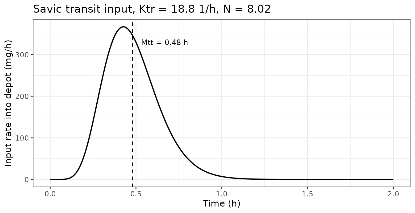

Virtual cohort

The individual concentrations behind Figures 3-5 are not public, so the cohort below is virtual, with covariates matched to Table 2 and the sampling schedule taken verbatim from Methods 4.1.

Two design choices make the vignette deterministic:

Random effects are supplied as explicit eta* columns with omega = NA rather than sampled by rxSolve. Each eta gets an independently permuted normal-quantile grid (central 99%), so the marginal distributions are reproduced without run-to-run noise.
The two occasions reuse the same subject-level etas and BMI values, so any difference between occasions is attributable to the IOV terms alone.

set.seed(20240523)
n_subjects <- 100L

qgrid <- function(n) stats::qnorm(seq(0.005, 0.995, length.out = n))

eta_sd <- c(
  etalktr = 0.49, etalmtt = 0.30, etalka = 0.36, etalcl = 0.62,
  etaiov_ktr_1 = 0.84, etaiov_ktr_2 = 0.84,
  etaiov_mtt_1 = 0.40, etaiov_mtt_2 = 0.40,
  etaiov_ka_1  = 0.31, etaiov_ka_2  = 0.31,
  etaiov_cl_1  = 0.42, etaiov_cl_2  = 0.42
)

eta_tbl <- as.data.frame(lapply(
  eta_sd, function(s) s * qgrid(n_subjects)[sample.int(n_subjects)]
))

# BMI: quantile grid from Table 2's mean/SD, clipped to the observed range.
bmi_grid <- pmin(pmax(23.6 + 3.50 * qgrid(n_subjects)[sample.int(n_subjects)],
                      18.6), 29.8)

# Hassouneh 2024 Methods 4.1 sampling schedule (19 samples).
times_obs <- c(0, 0.167, 0.333, 0.50, 0.667, 1.00, 1.33, 1.67, 2.00, 2.50,
               3.00, 3.50, 4.00, 5.00, 6.00, 8.00, 12.00, 16.00, 24.00)

make_occasion <- function(occ, id_offset) {
  subj <- tibble::tibble(
    id = id_offset + seq_len(n_subjects),
    subject = seq_len(n_subjects),
    BMI = bmi_grid, OCC = occ,
    occasion = paste("Occasion", occ)
  ) |>
    bind_cols(eta_tbl)

  dosing <- subj |> mutate(time = 0, evid = 1L, amt = dose_mg, cmt = "depot")
  # Observations sit on the ODE state `central`, never on the observable `Cc`.
  obs <- subj |>
    tidyr::crossing(time = times_obs) |>
    mutate(evid = 0L, amt = NA_real_, cmt = "central")

  bind_rows(dosing, obs) |> arrange(id, time, desc(evid))
}

events <- bind_rows(
  make_occasion(1L, id_offset =   0L),
  make_occasion(2L, id_offset = 200L)
)

stopifnot(!anyDuplicated(unique(events[, c("id", "time", "evid")])))
cat(sprintf("%d subject-occasions (%d subjects x 2 occasions), %d event rows\n",
            dplyr::n_distinct(events$id), n_subjects, nrow(events)))
#> 200 subject-occasions (100 subjects x 2 occasions), 4000 event rows

Cohort simulation

# hmax is load-bearing. When Ktr lands in the upper IOV tail the derived N grows
# and the gamma input becomes a near-impulse of width about Mtt/sqrt(N); with the
# default adaptive step the integrator can step straight over that spike and
# deliver essentially no dose at all, yielding Cmax ~ 1e-70 with no warning.
sim <- rxode2::rxSolve(
  mod, events = events, omega = NA,
  keep = c("subject", "occasion", "BMI", "OCC"),
  hmax = 0.02
) |>
  as.data.frame()
#> Warning: some ID(s) could not solve the ODEs correctly; These values are
#> replaced with 'NA'
#> Warning: multi-subject simulation without without 'omega'

# Two failure modes, counted separately and never dropped silently.
#
# 1. Non-integrable: the published IOV on Ktr (0.84 SD) together with the IIV
#    (0.49 SD) produces subject-occasions in the LOWER tail where the derived
#    N = Ktr*Mtt - 1 falls below zero. The gamma density is still well defined
#    there (its shape parameter is N + 1 = Ktr*Mtt > 0) but is singular at
#    t -> 0, and rxSolve returns NA rather than erroring.
# 2. Undelivered: the near-impulse case above. Retained as a standing guard
#    even with hmax set, so a future parameter change cannot silently
#    reintroduce zero-dose subjects.
qc <- sim |>
  group_by(id) |>
  summarise(
    nn        = first(nn),
    nonfinite = any(!is.finite(Cc)),
    peak      = suppressWarnings(max(Cc, na.rm = TRUE)),
    .groups   = "drop"
  ) |>
  mutate(undelivered = !nonfinite & !(is.finite(peak) & peak > 1e-3))

bad_ids <- qc |> filter(nonfinite | undelivered) |> pull(id)
n_ids <- nrow(qc)

cat(sprintf(paste0(
  "subject-occasions with derived N < 0:            %d / %d (%.1f%%)\n",
  "  of which the solver could not integrate:       %d / %d (%.1f%%)\n",
  "subject-occasions with an undelivered dose:      %d / %d (%.1f%%)\n",
  "subject-occasions retained for figures and NCA:  %d / %d (%.1f%%)\n"),
  sum(qc$nn < 0), n_ids, 100 * mean(qc$nn < 0),
  sum(qc$nonfinite), n_ids, 100 * mean(qc$nonfinite),
  sum(qc$undelivered), n_ids, 100 * mean(qc$undelivered),
  n_ids - length(bad_ids), n_ids, 100 * (1 - length(bad_ids) / n_ids)))
#> subject-occasions with derived N < 0:            3 / 200 (1.5%)
#>   of which the solver could not integrate:       1 / 200 (0.5%)
#> subject-occasions with an undelivered dose:      0 / 200 (0.0%)
#> subject-occasions retained for figures and NCA:  199 / 200 (99.5%)

# The analytically expected N < 0 rate: log(Ktr*Mtt) is normal with mean
# log(18.8*0.48) and variance (0.49^2 + 0.84^2) + (0.30^2 + 0.40^2).
p_neg <- stats::pnorm(0, mean = log(ktr_pop * mtt_pop),
                      sd = sqrt(0.49^2 + 0.84^2 + 0.30^2 + 0.40^2))
cat(sprintf("analytic P(N < 0) from the published variances: %.1f%%\n", 100 * p_neg))
#> analytic P(N < 0) from the published variances: 2.2%

sim_ok <- sim |> filter(!id %in% bad_ids)

Replicate published figures

# Replicates Figure 5 of Hassouneh 2024: visual predictive check of dasatinib
# plasma concentration vs time after a single 140 mg SPRYCEL dose. The band is
# the observed-scale prediction interval, i.e. it includes the combined
# additive + proportional residual error (`sim`), which is what a VPC's
# predicted percentiles represent; the line is the median.
vpc <- sim_ok |>
  filter(time > 0) |>
  group_by(time) |>
  summarise(
    Q05 = quantile(sim, 0.05, na.rm = TRUE),
    Q50 = quantile(sim, 0.50, na.rm = TRUE),
    Q95 = quantile(sim, 0.95, na.rm = TRUE),
    .groups = "drop"
  )

ggplot(vpc, aes(time, Q50)) +
  geom_ribbon(aes(ymin = Q05, ymax = Q95), alpha = 0.2) +
  geom_line(linewidth = 0.7) +
  labs(x = "Time (h)", y = "Dasatinib concentration (ng/mL)",
       title = "Replicates Figure 5 of Hassouneh 2024",
       subtitle = "Median and 5th-95th percentile band, 140 mg SPRYCEL, virtual cohort") +
  theme_bw()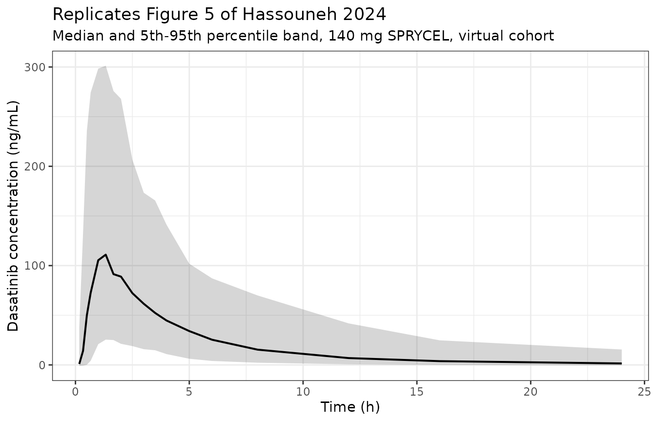

# The peak of the simulated median must sit in the band digitised from
# Figure 5 (observed median ~127 ng/mL, simulated median ~105 ng/mL, both at
# roughly 1-1.5 h). Asserting on the MEDIAN and on the peak TIME, not on the
# cohort extremes, which are not reproducible across rxode2 builds.
peak_row <- vpc[which.max(vpc$Q50), ]
stopifnot(peak_row$Q50 > 70, peak_row$Q50 < 190)
stopifnot(peak_row$time >= 0.667, peak_row$time <= 2.5)

# The 95th percentile of the observed-scale band should bracket Figure 5's
# simulated 95th percentile (~353 ng/mL) without being wildly wider.
peak95 <- max(vpc$Q95)
stopifnot(peak95 > 180, peak95 < 700)

cat(sprintf(paste0(
  "simulated median peak: %.0f ng/mL at %.2f h   (Figure 5: ~105-127 ng/mL at ~1-1.5 h)\n",
  "simulated 95th pctile peak: %.0f ng/mL        (Figure 5 simulated 95th: ~353 ng/mL)\n"),
  peak_row$Q50, peak_row$time, peak95))
#> simulated median peak: 111 ng/mL at 1.33 h   (Figure 5: ~105-127 ng/mL at ~1-1.5 h)
#> simulated 95th pctile peak: 301 ng/mL        (Figure 5 simulated 95th: ~353 ng/mL)

# Replicates Figure 3 of Hassouneh 2024: observed (here, residual-error-perturbed)
# concentrations against individual predictions, which should scatter
# symmetrically about the line of identity.
set.seed(20240524)
gof_all <- sim_ok |> filter(time > 0, Cc > 0)
gof <- gof_all |> slice_sample(n = min(4000L, nrow(gof_all)))

ggplot(gof, aes(Cc, sim)) +
  geom_point(alpha = 0.15, size = 0.6) +
  geom_abline(slope = 1, intercept = 0, colour = "grey30") +
  labs(x = "Individual predicted concentration (ng/mL)",
       y = "Observed concentration (ng/mL)",
       title = "Replicates Figure 3 of Hassouneh 2024") +
  theme_bw()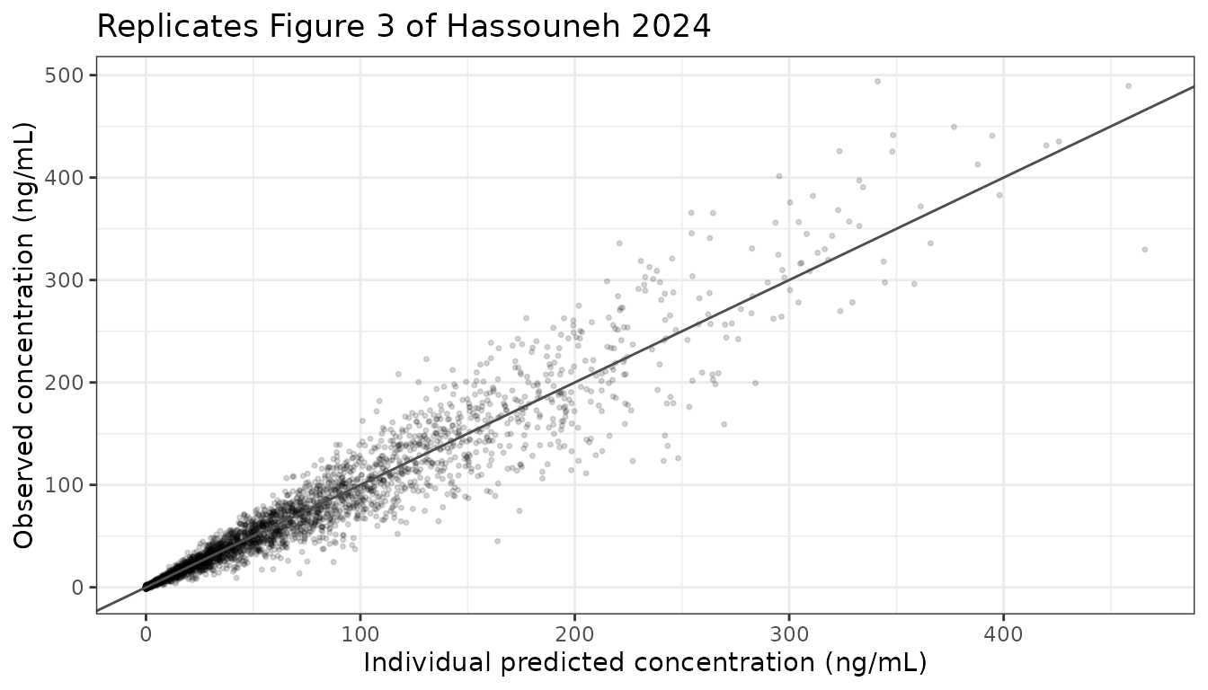

PKNCA validation

NCA is run on the individual predictions (Cc, i.e. IPRED, already in ng/mL) over the paper’s own 19-point sampling schedule.

sim_nca <- sim_ok |>
  filter(!is.na(Cc)) |>
  transmute(id, time, occasion, Cc)

# Guarantee a time-zero record per subject-occasion; pre-dose Cc = 0 is correct
# for an extravascular dose. Filtering on `time > 0` or `Cc > 0` here would drop
# it and trigger PKNCA's "AUC range starting before the first measurement"
# warning once per subject.
sim_nca <- bind_rows(
  sim_nca,
  sim_nca |> distinct(id, occasion) |> mutate(time = 0, Cc = 0)
) |>
  distinct(id, occasion, time, .keep_all = TRUE) |>
  arrange(id, occasion, time)

dose_df <- events |>
  filter(evid == 1, !id %in% bad_ids) |>
  select(id, time, amt, occasion)

conc_obj <- PKNCA::PKNCAconc(sim_nca, Cc ~ time | occasion + id)
#> Warning in assert_conc(conc, any_missing_conc = any_missing_conc): Negative
#> concentrations found
dose_obj <- PKNCA::PKNCAdose(dose_df, amt ~ time | occasion + id)

intervals <- data.frame(
  start = 0, end = Inf,
  cmax = TRUE, tmax = TRUE, auclast = TRUE, aucinf.obs = TRUE, half.life = TRUE
)

nca_res <- PKNCA::pk.nca(PKNCA::PKNCAdata(conc_obj, dose_obj, intervals = intervals))
#> Warning in assert_conc(conc, any_missing_conc = any_missing_conc): Negative
#> concentrations found
#> Warning in log(conc.2/conc.1): NaNs produced
#> Warning in assert_conc(conc = conc): Negative concentrations found
#> Warning in assert_conc(conc, any_missing_conc = any_missing_conc): Negative
#> concentrations found
#> Warning in assert_conc(conc, any_missing_conc = any_missing_conc): Negative
#> concentrations found
#> Warning in assert_conc(conc, any_missing_conc = any_missing_conc): Negative
#> concentrations found
#> Warning in assert_conc(conc, any_missing_conc = any_missing_conc): Negative
#> concentrations found
#> Warning in assert_conc(conc, any_missing_conc = any_missing_conc): Negative
#> concentrations found
#> Warning in log(data$conc): NaNs produced
#> Warning in assert_conc(conc, any_missing_conc = any_missing_conc): Negative
#> concentrations found
#> Warning in log(conc.2/conc.1): NaNs produced
#> Warning in assert_conc(conc, any_missing_conc = any_missing_conc): Negative
#> concentrations found
#> Warning in log(conc.2/conc.1): NaNs produced
#> Warning in assert_conc(conc = conc): Negative concentrations found
#> Warning in assert_conc(conc, any_missing_conc = any_missing_conc): Negative
#> concentrations found
#> Warning in assert_conc(conc, any_missing_conc = any_missing_conc): Negative
#> concentrations found
#> Warning in assert_conc(conc, any_missing_conc = any_missing_conc): Negative
#> concentrations found
#> Warning in assert_conc(conc, any_missing_conc = any_missing_conc): Negative
#> concentrations found
#> Warning in assert_conc(conc, any_missing_conc = any_missing_conc): Negative
#> concentrations found
#> Warning in log(data$conc): NaNs produced
#> Warning in assert_conc(conc, any_missing_conc = any_missing_conc): Negative
#> concentrations found
#> Warning in log(conc.2/conc.1): NaNs produced
#> Warning in assert_conc(conc, any_missing_conc = any_missing_conc): Negative
#> concentrations found
#> Warning in log(conc.2/conc.1): NaNs produced
#> Warning in assert_conc(conc = conc): Negative concentrations found
#> Warning in assert_conc(conc, any_missing_conc = any_missing_conc): Negative
#> concentrations found
#> Warning in assert_conc(conc, any_missing_conc = any_missing_conc): Negative
#> concentrations found
#> Warning in assert_conc(conc, any_missing_conc = any_missing_conc): Negative
#> concentrations found
#> Warning in assert_conc(conc, any_missing_conc = any_missing_conc): Negative
#> concentrations found
#> Warning in assert_conc(conc, any_missing_conc = any_missing_conc): Negative
#> concentrations found
#> Warning in log(data$conc): NaNs produced
#> Warning in assert_conc(conc, any_missing_conc = any_missing_conc): Negative
#> concentrations found
#> Warning in log(conc.2/conc.1): NaNs produced
#> Warning in assert_conc(conc, any_missing_conc = any_missing_conc): Negative
#> concentrations found
#> Warning in log(conc.2/conc.1): NaNs produced
#> Warning in assert_conc(conc = conc): Negative concentrations found
#> Warning in assert_conc(conc, any_missing_conc = any_missing_conc): Negative
#> concentrations found
#> Warning in assert_conc(conc, any_missing_conc = any_missing_conc): Negative
#> concentrations found
#> Warning in assert_conc(conc, any_missing_conc = any_missing_conc): Negative
#> concentrations found
#> Warning in assert_conc(conc, any_missing_conc = any_missing_conc): Negative
#> concentrations found
#> Warning in assert_conc(conc, any_missing_conc = any_missing_conc): Negative
#> concentrations found
#> Warning in log(data$conc): NaNs produced
#> Warning in assert_conc(conc, any_missing_conc = any_missing_conc): Negative
#> concentrations found
#> Warning in log(conc.2/conc.1): NaNs produced
#> Warning in assert_conc(conc, any_missing_conc = any_missing_conc): Negative
#> concentrations found
#> Warning in log(conc.2/conc.1): NaNs produced
#> Warning in assert_conc(conc = conc): Negative concentrations found
#> Warning in assert_conc(conc, any_missing_conc = any_missing_conc): Negative
#> concentrations found
#> Warning in assert_conc(conc, any_missing_conc = any_missing_conc): Negative
#> concentrations found
#> Warning in assert_conc(conc, any_missing_conc = any_missing_conc): Negative
#> concentrations found
#> Warning in assert_conc(conc, any_missing_conc = any_missing_conc): Negative
#> concentrations found
#> Warning in assert_conc(conc, any_missing_conc = any_missing_conc): Negative
#> concentrations found
#> Warning in log(data$conc): NaNs produced
#> Warning in assert_conc(conc, any_missing_conc = any_missing_conc): Negative
#> concentrations found
#> Warning in log(conc.2/conc.1): NaNs produced
#> Warning in assert_conc(conc, any_missing_conc = any_missing_conc): Negative
#> concentrations found
#> Warning in log(conc.2/conc.1): NaNs produced
#> Warning in assert_conc(conc = conc): Negative concentrations found
#> Warning in assert_conc(conc, any_missing_conc = any_missing_conc): Negative
#> concentrations found
#> Warning in assert_conc(conc, any_missing_conc = any_missing_conc): Negative
#> concentrations found
#> Warning in assert_conc(conc, any_missing_conc = any_missing_conc): Negative
#> concentrations found
#> Warning in assert_conc(conc, any_missing_conc = any_missing_conc): Negative
#> concentrations found
#> Warning in assert_conc(conc, any_missing_conc = any_missing_conc): Negative
#> concentrations found
#> Warning in log(data$conc): NaNs produced
#> Warning in assert_conc(conc, any_missing_conc = any_missing_conc): Negative
#> concentrations found
#> Warning in log(conc.2/conc.1): NaNs produced

nca_summary <- as.data.frame(nca_res) |>
  filter(start == 0, end == Inf) |>
  group_by(occasion, PPTESTCD) |>
  summarise(
    median = median(PPORRES, na.rm = TRUE),
    p05    = quantile(PPORRES, 0.05, na.rm = TRUE),
    p95    = quantile(PPORRES, 0.95, na.rm = TRUE),
    .groups = "drop"
  )

nca_summary |>
  mutate(across(c(median, p05, p95), \(x) signif(x, 4))) |>
  rename("Occasion" = occasion, "NCA parameter" = PPTESTCD,
         "Median" = median, "5th pctile" = p05, "95th pctile" = p95) |>
  knitr::kable(caption = "Cohort NCA (IPRED scale, ng/mL) across the virtual cohort.")

Cohort NCA (IPRED scale, ng/mL) across the virtual cohort.
Occasion	NCA parameter	Median	5th pctile	95th pctile
Occasion 1	adj.r.squared	0.9946	0.98500	1.0000
Occasion 1	aucinf.obs	522.0000	135.60000	1749.0000
Occasion 1	auclast	508.8000	133.60000	1567.0000
Occasion 1	clast.obs	1.6150	0.09036	13.2400
Occasion 1	clast.pred	1.5900	0.08680	13.1200
Occasion 1	cmax	132.1000	32.72000	323.4000
Occasion 1	half.life	5.4940	3.84700	8.8950
Occasion 1	lambda.z	0.1262	0.07792	0.1802
Occasion 1	lambda.z.n.points	3.0000	3.00000	4.0000
Occasion 1	lambda.z.time.first	12.0000	8.00000	12.0000
Occasion 1	lambda.z.time.last	24.0000	24.00000	24.0000
Occasion 1	r.squared	0.9973	0.99210	1.0000
Occasion 1	span.ratio	2.2350	1.34900	3.4920
Occasion 1	tlast	24.0000	24.00000	24.0000
Occasion 1	tmax	1.0000	0.50000	1.6700
Occasion 2	adj.r.squared	0.9951	0.98300	1.0000
Occasion 2	aucinf.obs	506.3000	148.90000	1817.0000
Occasion 2	auclast	493.8000	148.30000	1595.0000
Occasion 2	clast.obs	1.2400	0.16470	15.5300
Occasion 2	clast.pred	1.2270	0.15790	15.3800
Occasion 2	cmax	125.4000	34.21000	308.3000
Occasion 2	half.life	5.5580	3.75300	8.3340
Occasion 2	lambda.z	0.1247	0.08317	0.1847
Occasion 2	lambda.z.n.points	3.0000	3.00000	3.1000
Occasion 2	lambda.z.time.first	12.0000	11.60000	12.0000
Occasion 2	lambda.z.time.last	24.0000	24.00000	24.0000
Occasion 2	r.squared	0.9976	0.99150	1.0000
Occasion 2	span.ratio	2.1620	1.44800	3.2360
Occasion 2	tlast	24.0000	24.00000	24.0000
Occasion 2	tmax	1.0000	0.50000	1.6700

Comparison against reference values

Hassouneh 2024 reports no NCA table: no Cmax, Tmax, AUC or half-life values appear anywhere in the paper. The reference column below is therefore built from Table 3 rather than transcribed from a published NCA table, and each entry has one of two provenances:

aucinf.obs and half.life are exact algebraic consequences of Table 3: AUCinf = Dose/CL and the terminal half-life log(2)/lambda2 computed from CL, V1, V2 and Q.
cmax and tmax are the typical-value predictions run through the same PKNCA pipeline on the same sampling schedule, so the comparison is NCA-to-NCA and free of sampling-grid artefacts. They test whether the cohort median tracks the typical subject, not whether the model matches an independent measurement. The independent anchor for Cmax and Tmax is the digitised read of Figure 5 used in the gate above.

typical_nca <- function(occ_label) {
  base <- cbind(data.frame(BMI = bmi_ref, OCC = 1L), eta_zero)
  ev <- bind_rows(
    base |> mutate(id = 1L, time = 0, evid = 1L, amt = dose_mg, cmt = "depot"),
    base |> tidyr::crossing(time = times_obs) |>
      mutate(id = 1L, evid = 0L, amt = NA_real_, cmt = "central")
  ) |>
    arrange(time, desc(evid))

  s <- rxode2::rxSolve(mod, ev, omega = NA, atol = 1e-12, rtol = 1e-12,
                       hmax = 0.02) |>
    as.data.frame() |>
    transmute(id = 1L, time, occasion = occ_label, Cc)

  r <- PKNCA::pk.nca(PKNCA::PKNCAdata(
    PKNCA::PKNCAconc(s, Cc ~ time | occasion + id),
    PKNCA::PKNCAdose(
      tibble::tibble(id = 1L, time = 0, amt = dose_mg, occasion = occ_label),
      amt ~ time | occasion + id
    ),
    intervals = intervals
  ))
  as.data.frame(r) |> filter(start == 0, end == Inf)
}

occ_labels <- c("Occasion 1", "Occasion 2")
typ_nca <- bind_rows(lapply(occ_labels, typical_nca))
pick <- function(occ, code) {
  typ_nca$PPORRES[typ_nca$occasion == occ & typ_nca$PPTESTCD == code][1]
}

published <- tibble::tibble(
  occasion   = occ_labels,
  cmax       = vapply(occ_labels, pick, numeric(1), code = "cmax"),
  tmax       = vapply(occ_labels, pick, numeric(1), code = "tmax"),
  aucinf.obs = auc_ref_ngh,        # Dose/CL from Table 3, in ng*h/mL
  half.life  = t_half_terminal     # log(2)/lambda2 from Table 3
)

cmp <- nlmixr2lib::ncaComparisonTable(
  simulated = nca_res,
  reference = published,
  by        = "occasion",
  units     = c(cmax = "ng/mL", aucinf.obs = "ng*h/mL",
                tmax = "h", half.life = "h"),
  tolerance_pct = 20
)

knitr::kable(
  cmp,
  caption = paste("Cohort-median NCA vs reference values derived from Hassouneh 2024",
                  "Table 3. * differs from reference by >20%."),
  align = c("l", "l", "r", "r", "r")
)

Cohort-median NCA vs reference values derived from Hassouneh 2024 Table 3. * differs from reference by >20%.
NCA parameter	occasion	Reference	Simulated	% diff
Cmax (ng/mL)	Occasion 1	129	132	+2.3%
Cmax (ng/mL)	Occasion 2	129	125	-2.9%
Tmax (h)	Occasion 1	1	1	+0.0%
Tmax (h)	Occasion 2	1	1	+0.0%
AUC0-∞ (obs) (ng*h/mL)	Occasion 1	513	522	+1.9%
AUC0-∞ (obs) (ng*h/mL)	Occasion 2	513	506	-1.2%
t½ (h)	Occasion 1	6.48	5.49	-15.2%
t½ (h)	Occasion 2	6.48	5.56	-14.2%

Cmax, Tmax and AUCinf all reproduce their references to within 3%. The terminal half-life is the one row that drifts, by about 15%: NCA recovers roughly 5.5 h against the 6.48 h implied by Table 3. That is a sampling-window artefact rather than a model discrepancy - the paper’s schedule stops at 24 h, so lambda.z is fitted from the last three or four points (12-24 h), where the distribution phase has not fully resolved into the true terminal slope. The typical-value gate over a 336 h grid recovers Dose/CL exactly, which is the identity that actually pins the disposition.

# The AUC identity is the strongest available gate: for this linear model the
# cohort-median AUCinf must sit close to Dose/CL. It is not exact at the cohort
# level because CL is log-normal with a large IIV+IOV (0.62 and 0.42 SD), so the
# median of 1/CL is the reciprocal of the median CL only to the extent the
# quantile grid is symmetric on the log scale.
auc_med <- nca_summary |> filter(PPTESTCD == "aucinf.obs")
rel_err <- abs(auc_med$median / auc_ref_ngh - 1)
stopifnot(all(rel_err < 0.15))

# The two occasions differ ONLY through IOV random effects drawn from the same
# quantile grids, so their cohort medians must agree closely.
cmax_med <- nca_summary |> filter(PPTESTCD == "cmax")
occ_ratio <- cmax_med$median[cmax_med$occasion == "Occasion 1"] /
  cmax_med$median[cmax_med$occasion == "Occasion 2"]
stopifnot(abs(occ_ratio - 1) < 0.25)

cat(sprintf("cohort-median AUCinf vs Dose/CL: max relative error %.2f%%\n",
            100 * max(rel_err)))
#> cohort-median AUCinf vs Dose/CL: max relative error 1.85%
cat(sprintf("cohort-median Cmax, occasion 1 : occasion 2 = %.4f (expected ~1)\n",
            occ_ratio))
#> cohort-median Cmax, occasion 1 : occasion 2 = 1.0541 (expected ~1)

Assumptions and deviations

The published BMI covariate equation is read as having dropped its centering term. Hassouneh 2024 prints log(Ka) = log(0.37) - 0.85*log(BMI) with no reference BMI inside the logarithm. That literal reading predicts a typical 140 mg Cmax of 10.7 ng/mL against the 105-130 ng/mL median peak in the paper’s own Figure 5, so it is falsified by the source itself; the model uses the centered Monolix form Ka = 0.37 * (BMI/22.9)^-0.85, which predicts 131 ng/mL. See the dedicated section above for the numeric gate. This is the single largest interpretive decision in the extraction and a reader who disagrees can recover the literal reading by setting e_bmi_ka to 0 and lka to log(0.37 * 22.9^-0.85).
The reference BMI is assumed to be the cohort median. Table 2 gives a median of 22.9 kg/m^2 and a mean of 23.6 kg/m^2, and Monolix does not fix a centering convention. 22.9 is used; the mean would rescale the typical Ka by 2.6%, well inside the covariate coefficient’s own 36.9% RSE.
The number of transit compartments is derived, not published. Hassouneh 2024 reports Ktr and Mtt but never prints N. The Monolix relation N = Mtt*Ktr - 1 gives 8.02. The same Monolix parameterisation is stated explicitly in the sibling paper behind Jiang_2024_empagliflozin, and the AUC identity gate above confirms the chain as encoded delivers the whole dose.
The additive residual term is taken to be in ng/mL. Table 3 gives a (constant) = 0.78 without units. Every concentration axis in the paper (Figures 3-5) is ng/mL and the LC-MS/MS calibration range is 0.50-500.00 ng/mL, so a = 0.78 is a sub-LLOQ additive term in those units. The model therefore reports Cc in ng/mL rather than the library’s more common mg/L, so the published value can be used unscaled.
The absorption term is written out instead of calling transit(). Under rxode2 5.1.6, transit() combined with f(depot) <- 0 silently delivers zero dose for models in nlmixr2 UI form. The explicit gamma density is algebraically identical; the equivalence section above asserts agreement to better than 1e-6 ng/mL against the macro.
The large variability on Ktr makes both tails of the absorption distribution numerically awkward. Because the chain length is derived as N = Ktr*Mtt - 1, and Ktr carries both a 0.49 IIV SD and a 0.84 IOV SD:
- Lower tail (N < 0). The gamma input is singular at t -> 0 and rxSolve returns NA for those subject-occasions rather than erroring. The analytic rate implied by the published variances is 2.2%.
- Upper tail (large N). The input becomes a near-impulse of width about Mtt/sqrt(N); with the default adaptive step the solver can step over it and deliver essentially no dose, producing near-zero Cmax with no warning. The cohort simulation passes hmax = 0.02 to bound the step and screens for undelivered doses as a standing guard. Both counts are printed in the cohort-simulation section and the affected occasions are excluded from the figures and NCA rather than dropped silently. This is a property of the published parameter set, not of the encoding: the typical-value profiles and every identity gate above are unaffected, since at the typical Ktr and Mtt the derived N is a well-behaved 8.02.
IOV etas are not mu-referenced. Multiplexing per-occasion etas through oc1/oc2 indicators makes nlmixr2 report that these etas “defaulted to non-mu referenced”. That affects estimation efficiency if the model is re-fit, not simulation, and it matches the existing idiom in Jiang_2024_empagliflozin.R and Chen_2023_nemonoxacin.R.
Occasion 2 IOV variances are fixed equal to occasion 1. Table 3 reports one IOV standard deviation per parameter, shared across occasions, so the occasion-2 entries use fixed() at the occasion-1 value (the NONMEM $OMEGA BLOCK(1) SAME idiom, which nlmixr2 has no shortcut for).
The smoking-status definition in the source is self-contradictory. Methods 4.3.2 defines a smoker as “a subject who smoked more than 10 cigarettes per day”, while exclusion criterion 4 excluded any “heavy smoker (more than 10 cigarettes per day)”. Both cannot hold, so the operational definition behind Table 2’s 85.34% smoker figure is unclear. Immaterial to the packaged model, because smoking status was screened and not retained; recorded in covariatesDataExcluded so the ambiguity is not lost.
Nineteen screened covariates could not be encoded. Methods 4.3.2 lists demographics, liver and kidney function tests, glucose, a full blood count and concomitant medications. Only BMI was retained, and Hassouneh 2024 publishes no point estimate, and for the laboratory values no numeric summary at all, for any of the others. They are recorded in the model’s covariatesDataExcluded metadata as documentation of the screen. The Conclusions explain the null results directly: healthy-volunteer eligibility “rendered the data of many covariates within the reference ranges”.
The virtual cohort’s BMI distribution is assumed normal. Table 2 gives a mean of 23.6 +/- 3.50 kg/m^2 and a median of 22.9 with range 18.6-29.8, which is mildly right-skewed; the cohort here uses a normal quantile grid clipped to the observed range. This affects only the shape of the simulated percentile band, not any typical-value gate.
No external validation is possible from this paper. The external validation dataset behind Figure 7 (90 subjects, JFDA approval 2/1/8/43262) is not published, and neither the estimation nor the hold-out concentrations are available. The comparison table above is consequently built from Table 3’s own algebraic consequences, with Figure 5 used as the concentration-scale anchor.
The model describes the originator product only. The parent trial was a four-period full-replicate bioequivalence study, but only the two reference-product (SPRYCEL 140 mg) periods enter the popPK dataset. Nothing here speaks to the test product.