Vitacoxib in cats (Wang 2020) • nlmixr2lib

Model and source

mod <- rxode2::rxode2(readModelDb("Wang_2020_vitacoxib_cat"))
#> ℹ parameter labels from comments will be replaced by 'label()'

Citation: Wang J, Schneider BK, Xiao H, Qiu J, Gong X, Seo Y-J, Li J, Mochel JP, Cao X. Non-Linear Mixed-Effects Pharmacokinetic Modeling of the Novel COX-2 Selective Inhibitor Vitacoxib in Cats. Front Vet Sci. 2020;7:554033. doi:10.3389/fvets.2020.554033.
Description: Preclinical/clinical veterinary (cat). Two-compartment population PK model for the COX-2 selective inhibitor vitacoxib in healthy neutered domestic shorthair cats, pooling intravenous and single- and multiple-dose oral data from six studies. Oral absorption is a parallel mixed-order input: a fraction Fr of the bioavailable dose is absorbed first-order through a depot (ka = 0.13 1/h) and the remainder enters the central compartment by a zero-order process of duration Tk0 = 3.76 h; oral bioavailability 57.8%. Clearance is per kg body weight (Table 2 prints 0.11 ‘L/h’; the paper’s Figure 6 simulations and companion NCA identify it as L/h/kg) and body weight is a power covariate on the central volume of distribution (Wang 2020)
Article: https://doi.org/10.3389/fvets.2020.554033

Vitacoxib is a highly selective cyclooxygenase-2 (COX-2) inhibitor registered for dogs in China. Wang 2020 pooled six pharmacokinetic studies in 16 healthy cats to build a population PK model in Monolix 2019R2 and then used deterministic simulations to relate oral and intravenous dose to the time that plasma concentrations stay above in-vitro whole-blood COX-1 and COX-2 inhibitory concentrations.

Population

Sixteen healthy, neutered, domestic shorthair laboratory cats, 1-3 years old, body weight 2.9 +/- 0.78 kg (Methods “Animals”), in two groups of eight (Table 1):

Study	Cats	Feeding	Route	Dose
1	IDs 9-16	12 h fast	oral	2 mg/kg single
2	IDs 9-16	12 h fast	i.v.	2 mg/kg single
3	IDs 9-16	2 h after feeding	oral	2 mg/kg single
4	IDs 1-8	12 h fast	oral	1 mg/kg single
5	IDs 1-8	12 h fast	oral	4 mg/kg single
6	IDs 9-16	12 h fast	oral	2 mg/kg daily x 7 days

Plasma was assayed by UPLC-MS/MS (LLOQ 0.5 ng/mL); below-LLOQ data were handled with the Monolix equivalent of the NONMEM M3 method. The sex split is not reported.

str(readModelDb("Wang_2020_vitacoxib_cat")()$population)
#> List of 11
#>  $ species       : chr "cat (domestic shorthair; Felis catus)"
#>  $ n_subjects    : int 16
#>  $ n_studies     : int 6
#>  $ age_range     : chr "1-3 years"
#>  $ weight_range  : chr "2.9 +/- 0.78 kg (mean +/- SD)"
#>  $ weight_mean   : chr "2.9 kg"
#>  $ sex_female_pct: num NA
#>  $ disease_state : chr "Healthy neutered domestic shorthair laboratory cats"
#>  $ dose_range    : chr "1, 2 and 4 mg/kg single oral dose; 2 mg/kg single i.v. dose; 2 mg/kg oral once daily for 7 days"
#>  $ regions       : chr "China (China Agricultural University, Beijing)"
#>  $ notes         : chr "Methods 'Animals' and Table 1. Two groups of eight cats: IDs 9-16 received Study 1 (2 mg/kg p.o. fasted), Study"| __truncated__

Structural model

Figure 1 and Results “PK Model Evaluation”: a two-compartment mammillary model with simultaneous first- and zero-order oral absorption. Of the bioavailable oral dose (F = 57.8%), a fraction Fr = 0.20 is absorbed first-order through a depot (ka = 0.13 1/h) and 1 - Fr enters the central compartment by a zero-order input of duration Tk0 = 3.76 h. This is the same parallel-input structure the authors cite from the robenacoxib cat model (Pelligand 2016, Pelligand_2016_robenacoxib_cat).

Because rxode2 applies one bioavailability per compartment rather than per administration type, the canonical ROUTE_IV indicator selects which bioavailability applies to a dose placed in central:

cat(paste(mod$modelDesc, collapse = "\n"))
#> rxode2-based free-form 3-cmt ODE model

An oral administration is two dose records at the same time: a bolus into depot and a rate = -2 record into central, both with ROUTE_IV = 0. An intravenous administration is one plain bolus into central with ROUTE_IV = 1; that record carries no rate, so dur(central) is ignored.

Source trace

Equation / parameter	Value	Source location
Two-compartment disposition, parallel zero- + first-order oral input	n/a	Figure 1; Results “PK Model Evaluation”
`lcl` (CL)	0.11 L/h/kg (printed “L/h”)	Table 2 “Systemic Clearance”; per-kg reading justified below
`lvc` (V1)	2.88 L	Table 2 “Central compartment volume of distribution”
`lvp` (V2)	0.54 L	Table 2 “Peripheral compartment volume of distribution”
`lq` (Q)	0.52 L/h	Table 2 “Inter-compartmental clearance”
`lka` (Ka)	0.13 1/h	Table 2 “First-order absorption rate constant (P.O)”
`ld1` (Tk0)	3.76 h	Table 2 “Zero-order absorption rate constant (P.O)” (a duration, unit h)
`logitfdepot` (F)	0.578	Table 2 “Bioavailability (P.O)”
`logitffo` (Fr)	0.20	Table 2 “Fraction absorbed through 1st order”
`e_wt_vc`	0.41 on log(WT / 2.9)	Table 2 “Bodyweight effect on V1”; Equation 2; Methods “Inclusion of Covariate Relationships”
`etalka`, `etalq`	0.01, fixed	Table 2 CV 10.0%; Results “Parameter Estimates”: set to 0.1
`etald1`, `etalvc`, `etalvp`, `etalcl`	CV 31.5, 37.4, 109, 46.0%	Table 2 CV column, `log(1 + CV^2)`
`etalogitffo`, `etalogitfdepot`	SD 0.08, 0.265 (logit scale)	Table 2 CV column
`propSd`	0.30	Table 2 “Proportional error constant”

Typical-value verification

With the random effects zeroed, closed-form identities must hold. These compare a solve against its own analytic solution, so the tolerances are tight.

wt_ref <- 2.9 # Methods "Animals": mean body weight

make_events <- function(id, dose_mgkg, route_iv, wt = wt_ref, times = seq(0, 240, by = 0.05)) {
  amt <- dose_mgkg * wt
  if (route_iv == 1) {
    dosing <- data.frame(id = id, time = 0, evid = 1L, cmt = "central", amt = amt, rate = 0)
  } else {
    dosing <- data.frame(
      id = id, time = 0, evid = 1L, cmt = c("depot", "central"),
      amt = amt, rate = c(0, -2)
    )
  }
  obs <- data.frame(id = id, time = times, evid = 0L, cmt = "central", amt = NA_real_, rate = NA_real_)
  out <- rbind(dosing, obs)
  out$WT <- wt
  out$ROUTE_IV <- route_iv
  out
}

mod_typ <- rxode2::zeroRe(mod)
ev_typ <- rbind(make_events(1, 2, 1), make_events(2, 2, 0))
sim_typ <- as.data.frame(rxode2::rxSolve(mod_typ, ev_typ, returnType = "data.frame"))
#> ℹ omega/sigma items treated as zero: 'etalka', 'etald1', 'etalogitffo', 'etalvc', 'etalvp', 'etalq', 'etalcl', 'etalogitfdepot'
#> Warning: multi-subject simulation without without 'omega'

trap <- function(t, y) sum(diff(t) * (head(y, -1) + tail(y, -1)) / 2)
typ <- sim_typ |>
  dplyr::group_by(id) |>
  dplyr::summarise(c0 = Cc[time == 0], cmax = max(Cc), tmax = time[which.max(Cc)], auc = trap(time, Cc))

CL <- 0.11 * wt_ref
V1 <- 2.88
V2 <- 0.54
FORAL <- 0.578
dose <- 2 * wt_ref
checks <- data.frame(
  Identity = c(
    "IV C0 = Dose/V1 (ng/mL)",
    "IV AUC0-240h ~ Dose/CL (ng*h/mL)",
    "Oral AUC0-240h ~ F*Dose/CL (ng*h/mL)"
  ),
  Analytic = c(dose / V1 * 1000, dose / CL * 1000, FORAL * dose / CL * 1000),
  Simulated = c(typ$c0[1], typ$auc[1], typ$auc[2])
) |>
  dplyr::mutate("% diff" = 100 * (Simulated - Analytic) / Analytic)
knitr::kable(checks, digits = 3)

Identity	Analytic	Simulated	% diff
IV C0 = Dose/V1 (ng/mL)	2013.889	2013.889	0.000
IV AUC0-240h ~ Dose/CL (ng*h/mL)	18181.818	18181.940	0.001
Oral AUC0-240h ~ FDose/CL (ngh/mL)	10509.091	10509.035	-0.001


stopifnot(
  abs(typ$c0[1] / (dose / V1 * 1000) - 1) < 1e-6,
  abs(typ$auc[1] / (dose / CL * 1000) - 1) < 0.005,
  # Blind to the Fr split and Tk0 (total exposure only), but goes red if either
  # f() multiplier is wrong or the zero-order record is dropped/double-counted.
  abs(typ$auc[2] / (FORAL * dose / CL * 1000) - 1) < 0.005,
  # Abstract / Results: VSS = 3.42 L = V1 + V2.
  abs((V1 + V2) - 3.42) < 1e-9
)

The absorption split and the zero-order duration are not visible in total exposure, so they are pinned separately: dosing only the first-order record must give F*Fr of the oral AUC, and the zero-order record alone must peak at Tk0.

ev_split <- rbind(
  make_events(1, 2, 0)[-2, ], # depot record only
  make_events(2, 2, 0)[-1, ] # zero-order central record only
)
ev_split$id <- rep(1:2, each = nrow(ev_split) / 2)
sim_split <- as.data.frame(rxode2::rxSolve(mod_typ, ev_split, returnType = "data.frame"))
#> ℹ omega/sigma items treated as zero: 'etalka', 'etald1', 'etalogitffo', 'etalvc', 'etalvp', 'etalq', 'etalcl', 'etalogitfdepot'
#> Warning: multi-subject simulation without without 'omega'
split <- sim_split |>
  dplyr::group_by(id) |>
  dplyr::summarise(auc = trap(time, Cc), tmax = time[which.max(Cc)])
stopifnot(
  abs(split$auc[1] / (FORAL * 0.20 * dose / CL * 1000) - 1) < 0.005,
  abs(split$auc[2] / (FORAL * 0.80 * dose / CL * 1000) - 1) < 0.005,
  abs(split$tmax[2] - 3.76) <= 0.05
)
split
#> # A tibble: 2 × 3
#>      id   auc  tmax
#>   <int> <dbl> <dbl>
#> 1     1 2102.  8.9 
#> 2     2 8407.  3.75

Clearance is per kg body weight

Table 2 prints CL = 0.11 L/h and the Abstract “110 ml/h”. Encoded that way, the model cannot reproduce the paper’s own Figure 6, which the authors simulated deterministically from this final model with mlxR (IIV and residual error fixed to zero). Figure 6 plots the time above four in-vitro targets against dose; its curves were read at the grid lines by the maintainers:

fig6 <- rbind(
  data.frame(target = "COX-2 IC80", conc = 313.0, route_iv = 1, dose = c(1, 2, 4, 8), fig = c(11, 19, 27, 35)),
  data.frame(target = "COX-2 IC80", conc = 313.0, route_iv = 0, dose = c(1, 2, 4, 8), fig = c(5, 14, 23.5, 32)),
  data.frame(target = "COX-1 IC10", conc = 911.3, route_iv = 1, dose = c(2, 4, 8), fig = c(8, 15, 23)),
  data.frame(target = "COX-1 IC10", conc = 911.3, route_iv = 0, dose = c(4, 8), fig = c(8.5, 18.5)),
  data.frame(target = "COX-2 IC90", conc = 556.5, route_iv = 0, dose = c(2, 4, 8), fig = c(5, 15.5, 25))
)

The model is solved at the mean weight of 2.9 kg in two variants: as encoded (CL = 0.11 L/h/kg x 2.9 kg = 0.319 L/h) and with the printed absolute value (CL = 0.11 L/h, obtained by dividing the per-kg value by the weight).

time_above <- function(model, doses, routes, conc) {
  grid <- unique(data.frame(dose = doses, route_iv = routes))
  grid$id <- seq_len(nrow(grid))
  ev <- do.call(rbind, Map(make_events, grid$id, grid$dose, grid$route_iv))
  s <- as.data.frame(rxode2::rxSolve(model, ev, returnType = "data.frame"))
  s <- dplyr::left_join(s, grid, by = "id")
  mapply(function(d, r, cc) {
    x <- s[s$dose == d & s$route_iv == r, ]
    stopifnot(nrow(x) > 1000) # a lookup that matched nothing must not pass
    sum(x$Cc > cc) * 0.05
  }, doses, routes, conc)
}
mod_printed <- rxode2::ini(mod_typ, lcl = log(0.11 / wt_ref))
#> ℹ change initial estimate of `lcl` to `-3.27198565018215`
fig6$per_kg <- time_above(mod_typ, fig6$dose, fig6$route_iv, fig6$conc)
#> ℹ omega/sigma items treated as zero: 'etalka', 'etald1', 'etalogitffo', 'etalvc', 'etalvp', 'etalq', 'etalcl', 'etalogitfdepot'
#> Warning: multi-subject simulation without without 'omega'
fig6$printed <- time_above(mod_printed, fig6$dose, fig6$route_iv, fig6$conc)
#> ℹ omega/sigma items treated as zero: 'etalka', 'etald1', 'etalogitffo', 'etalvc', 'etalvp', 'etalq', 'etalcl', 'etalogitfdepot'
#> Warning: multi-subject simulation without without 'omega'
rmse <- function(x) sqrt(mean((x - fig6$fig)^2))

fig6 |>
  dplyr::mutate(route = ifelse(route_iv == 1, "IV", "PO")) |>
  dplyr::select(target, route, dose, fig, per_kg, printed) |>
  dplyr::rename(
    "Target" = target, "Route" = route, "Dose (mg/kg)" = dose,
    "Figure 6 (h)" = fig, "CL 0.11 L/h/kg (h)" = per_kg, "CL 0.11 L/h (h)" = printed
  ) |>
  knitr::kable(digits = 1)

Target	Route	Dose (mg/kg)	Figure 6 (h)	CL 0.11 L/h/kg (h)	CL 0.11 L/h (h)
COX-2 IC80	IV	1	11.0	10.5	30.9
COX-2 IC80	IV	2	19.0	18.0	52.5
COX-2 IC80	IV	4	27.0	25.6	74.2
COX-2 IC80	IV	8	35.0	33.2	95.9
COX-2 IC80	PO	1	5.0	2.5	12.8
COX-2 IC80	PO	2	14.0	13.2	37.3
COX-2 IC80	PO	4	23.5	22.3	59.9
COX-2 IC80	PO	8	32.0	30.8	81.8
COX-1 IC10	IV	2	8.0	6.4	19.1
COX-1 IC10	IV	4	15.0	14.0	40.8
COX-1 IC10	IV	8	23.0	21.6	62.5
COX-1 IC10	PO	4	8.5	7.7	24.6
COX-1 IC10	PO	8	18.5	17.5	47.8
COX-2 IC90	PO	2	5.0	4.4	17.3
COX-2 IC90	PO	4	15.5	14.8	41.2
COX-2 IC90	PO	8	25.0	23.8	63.6


c(rmse_per_kg = rmse(fig6$per_kg), rmse_printed = rmse(fig6$printed))
#>  rmse_per_kg rmse_printed 
#>     1.274694    33.167814
stopifnot(
  rmse(fig6$per_kg) < 3,
  rmse(fig6$printed) > 20
)

The per-kg reading reproduces all 16 digitised points to an RMSE of about 1 h; the printed unit misses them by more than a day. Only clearance needs rescaling: the dose at which each curve leaves zero is set by the peak concentration, and the intravenous thresholds (for example about 0.85 mg/kg for COX-1 IC10) put C0 / dose at about 1,050 ng/mL per mg/kg, which is 2.9 / 2.88 x 1000 = 1,007 – i.e. V1 = 2.88 L is an absolute volume. Independently, the companion non-compartmental analysis of the same Study 2 intravenous data (Wang 2019, J Vet Pharmacol Ther 42:294, ref. 16 of the paper) reports CL = 95.22 +/- 23.53 ml/kg/h and Vd = 1,264 +/- 344 ml/kg – about 0.28 L/h and 3.7 L for a 2.9 kg cat, matching the per-kg clearance and the absolute volumes.

dose_grid <- c(0.1, seq(0.25, 8, by = 0.25))
curves <- expand.grid(dose = dose_grid, route_iv = c(0, 1), conc = c(313.0, 556.5, 911.3, 1467.8))
curves$hours <- time_above(mod_typ, curves$dose, curves$route_iv, curves$conc)
#> ℹ omega/sigma items treated as zero: 'etalka', 'etald1', 'etalogitffo', 'etalvc', 'etalvp', 'etalq', 'etalcl', 'etalogitfdepot'
#> Warning: multi-subject simulation without without 'omega'
curves$target <- factor(curves$conc,
  levels = c(911.3, 1467.8, 313.0, 556.5),
  labels = c("COX-1 IC10", "COX-1 IC20", "COX-2 IC80", "COX-2 IC90")
)
ggplot(curves, aes(dose, hours, colour = ifelse(route_iv == 1, "IV", "PO"))) +
  geom_line() +
  geom_point(
    data = fig6 |> dplyr::mutate(target = factor(target, levels = levels(curves$target))),
    aes(y = fig), shape = 1
  ) +
  facet_wrap(~target) +
  labs(
    x = "Dose (mg/kg)", y = "Time above target (h)", colour = NULL,
    caption = "Lines: model, typical 2.9 kg cat. Circles: digitised from Figure 6 of Wang 2020."
  )

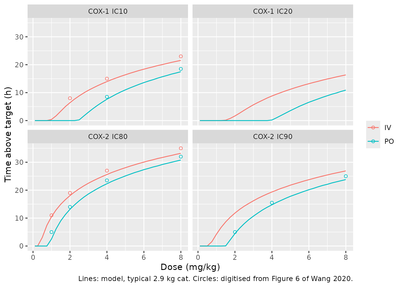
Replicates Figure 6 of Wang 2020. Results “Model Simulations” states that 2 mg/kg orally stays above the COX-2 IC80 for about 12 h without reaching the COX-1 IC10, and 4 mg/kg for about 24 h:

claims <- time_above(mod_typ, c(2, 2, 4), c(0, 0, 0), c(313.0, 911.3, 313.0))
#> ℹ omega/sigma items treated as zero: 'etalka', 'etald1', 'etalogitffo', 'etalvc', 'etalvp', 'etalq', 'etalcl', 'etalogitfdepot'
#> Warning: multi-subject simulation without without 'omega'
claims
#> [1] 13.15  0.00 22.30
stopifnot(
  claims[2] == 0,
  abs(claims[1] - 12) < 3,
  abs(claims[3] - 24) < 3
)

Stochastic simulation of the six studies

Each study period is simulated as a separate set of animals, because the random effects in Table 2 are between-occasion (study-period) variability. Weights are drawn from a normal distribution with the reported mean and SD, with draws outside 1.5-5 kg rejected and redrawn.

rxode2::rxSetSeed(20200924)
n_per_arm <- 100
draw_wt <- function(n) {
  w <- numeric(0)
  while (length(w) < n) {
    x <- stats::rnorm(n, 2.9, 0.78)
    w <- c(w, x[x >= 1.5 & x <= 5])
  }
  w[seq_len(n)]
}
arms <- data.frame(
  study = c("Study 4: 1 mg/kg PO", "Study 1: 2 mg/kg PO", "Study 5: 4 mg/kg PO", "Study 2: 2 mg/kg IV"),
  dose = c(1, 2, 4, 2),
  route_iv = c(0, 0, 0, 1)
)
obs_times <- sort(unique(c(0, 0.08, 0.25, 0.33, 0.5, 0.67, 1, 2, 3, 4, 5, 6, 8, 10, 12, 24, 36, 48)))
ev_sd <- do.call(rbind, lapply(seq_len(nrow(arms)), function(a) {
  wts <- draw_wt(n_per_arm)
  do.call(rbind, lapply(seq_len(n_per_arm), function(i) {
    e <- make_events((a - 1) * n_per_arm + i, arms$dose[a], arms$route_iv[a], wt = wts[i], times = obs_times)
    e$study <- arms$study[a]
    e
  }))
}))
sim_sd <- as.data.frame(rxode2::rxSolve(mod, ev_sd, returnType = "data.frame", keep = c("study", "WT")))

sim_sd[sim_sd$time > 0, ] |>
  dplyr::group_by(study, time) |>
  dplyr::summarise(
    p05 = quantile(Cc, 0.05), p50 = median(Cc), p95 = quantile(Cc, 0.95),
    .groups = "drop"
  ) |>
  ggplot(aes(time, p50)) +
  geom_ribbon(aes(ymin = p05, ymax = p95), alpha = 0.25) +
  geom_line() +
  scale_y_log10() +
  facet_wrap(~study) +
  labs(x = "Time (h)", y = "Vitacoxib (ng/mL)", caption = "Median and 90% interval of 100 simulated cats per study")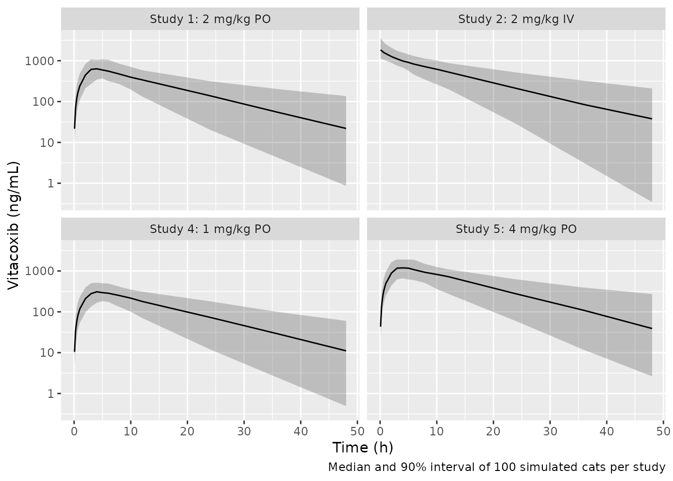

PKNCA validation

conc <- sim_sd |>
  dplyr::filter(!is.na(Cc)) |>
  dplyr::mutate(treatment = study) |>
  dplyr::select(id, time, Cc, treatment, WT)
dose_df <- ev_sd |>
  dplyr::filter(evid == 1) |>
  dplyr::group_by(id, study, WT) |>
  dplyr::summarise(time = 0, amt = sum(amt), .groups = "drop") |>
  dplyr::rename(treatment = study)

conc_obj <- PKNCA::PKNCAconc(conc, Cc ~ time | treatment + id)
dose_obj <- PKNCA::PKNCAdose(dose_df, amt ~ time | treatment + id)
intervals <- data.frame(
  start = 0, end = Inf, cmax = TRUE, tmax = TRUE, aucinf.obs = TRUE,
  half.life = TRUE, cl.obs = TRUE
)
nca <- PKNCA::pk.nca(PKNCA::PKNCAdata(conc_obj, dose_obj, intervals = intervals))
nca_res <- as.data.frame(nca$result)
summary(nca)
#>  start end           treatment   N        cmax                 tmax   half.life
#>      0 Inf Study 1: 2 mg/kg PO 100  681 [37.9]    4.00 [2.00, 8.00] 10.3 [5.50]
#>      0 Inf Study 2: 2 mg/kg IV 100 1920 [38.8] 0.000 [0.000, 0.000] 10.5 [6.23]
#>      0 Inf Study 4: 1 mg/kg PO 100  342 [33.2]    4.00 [2.00, 8.00] 10.1 [5.24]
#>      0 Inf Study 5: 4 mg/kg PO 100 1330 [32.5]    4.00 [2.00, 8.00] 10.4 [5.63]
#>    aucinf.obs          cl.obs
#>  10400 [42.9]  0.00111 [50.9]
#>  18800 [42.0] 0.000294 [50.8]
#>   5340 [44.7]  0.00109 [54.1]
#>  20500 [45.6]  0.00109 [52.3]
#> 
#> Caption: cmax, aucinf.obs, cl.obs: geometric mean and geometric coefficient of variation; tmax: median and range; half.life: arithmetic mean and standard deviation; N: number of subjects

The companion NCA paper (Wang 2019, ref. 16 of the article) analysed the same Study 1-5 data and reports mean Cmax of 352.30, 750.26 and 936.97 ng/mL at 1, 2 and 4 mg/kg orally, a Tmax of about 4.7 h at 2 mg/kg, and an i.v. clearance of 95.22 ml/kg/h.

# Raw PKNCA clearance is mg / (ng*h/mL) = 1000 L/h; x 1e6 / WT gives ml/h/kg.
wt_by_id <- dose_df |> dplyr::select(id, WT)
sim_long <- nca_res |>
  dplyr::filter(PPTESTCD %in% c("cmax", "tmax", "cl.obs")) |>
  dplyr::left_join(wt_by_id, by = "id") |>
  dplyr::mutate(PPORRES = ifelse(PPTESTCD == "cl.obs", PPORRES * 1e6 / WT, PPORRES)) |>
  dplyr::select(treatment, PPTESTCD, PPORRES)
ref_long <- data.frame(
  treatment = c(arms$study[1:3], arms$study[2], arms$study[4]),
  PPTESTCD = c("cmax", "cmax", "cmax", "tmax", "cl.obs"),
  PPORRES = c(352.30, 750.26, 936.97, 4.7, 95.22)
)
cmp <- nlmixr2lib::ncaComparisonTable(
  sim_long, ref_long,
  by = "treatment",
  units = c(cmax = "ng/mL", tmax = "h", cl.obs = "ml/h/kg")
)
# After an i.v. dose the observed clearance is CL, not CL/F.
cmp[[1]] <- sub("^CL/F", "CL", cmp[[1]])
knitr::kable(cmp, caption = "Simulated median vs. companion NCA mean (Wang 2019).")

Simulated median vs. companion NCA mean (Wang 2019).
NCA parameter	treatment	Reference	Simulated	% diff
Cmax (ng/mL)	Study 4: 1 mg/kg PO	352	343	-2.8%
Cmax (ng/mL)	Study 1: 2 mg/kg PO	750	676	-9.9%
Cmax (ng/mL)	Study 5: 4 mg/kg PO	937	1360	+45.0%*
Tmax (h)	Study 1: 2 mg/kg PO	4.7	4	-14.9%
CL (ml/h/kg)	Study 2: 2 mg/kg IV	95.2	106	+11.7%

if (!is.null(attr(cmp, "footnote"))) cat(attr(cmp, "footnote"))
#> * differs from reference by more than ±20%.

sim_med <- sim_long |>
  dplyr::group_by(treatment, PPTESTCD) |>
  dplyr::summarise(sim = median(PPORRES, na.rm = TRUE), .groups = "drop")
chk <- dplyr::inner_join(ref_long, sim_med, by = c("treatment", "PPTESTCD")) |>
  dplyr::mutate(pct_diff = 100 * (sim - PPORRES) / PPORRES)
stopifnot(
  nrow(chk) == 5,
  # Structural: a per-kg vs absolute clearance mix-up moves this by ~2.9x.
  abs(chk$pct_diff[chk$PPTESTCD == "cl.obs"]) < 30,
  # Centre of the oral peaks across the three dose levels.
  abs(median(chk$pct_diff[chk$PPTESTCD == "cmax"])) < 35
)

The simulated 1 and 2 mg/kg oral peaks lie close to the NCA means. The 4 mg/kg NCA mean (936.97 ng/mL) is less than dose-proportional to the 2 mg/kg one although the companion paper reports linear scaling; the model, which is linear, predicts a higher peak at 4 mg/kg.

Multiple dosing (Study 6)

ev_md <- rbind(
  data.frame(
    id = 1, time = rep(24 * (0:6), each = 2), evid = 1L,
    cmt = rep(c("depot", "central"), 7), amt = 2 * wt_ref, rate = rep(c(0, -2), 7)
  ),
  data.frame(
    id = 1, time = seq(0, 192, by = 0.25), evid = 0L, cmt = "central",
    amt = NA_real_, rate = NA_real_
  )
)
ev_md$WT <- wt_ref
ev_md$ROUTE_IV <- 0
sim_md <- as.data.frame(rxode2::rxSolve(mod_typ, ev_md, returnType = "data.frame"))
#> ℹ omega/sigma items treated as zero: 'etalka', 'etald1', 'etalogitffo', 'etalvc', 'etalvp', 'etalq', 'etalcl', 'etalogitfdepot'
ggplot(sim_md, aes(time, Cc)) +
  geom_line() +
  geom_hline(yintercept = c(313.0, 911.3), linetype = 2) +
  labs(
    x = "Time (h)", y = "Vitacoxib (ng/mL)",
    caption = "Typical 2.9 kg cat, 2 mg/kg orally once daily for 7 days; dashed: COX-2 IC80 and COX-1 IC10"
  )

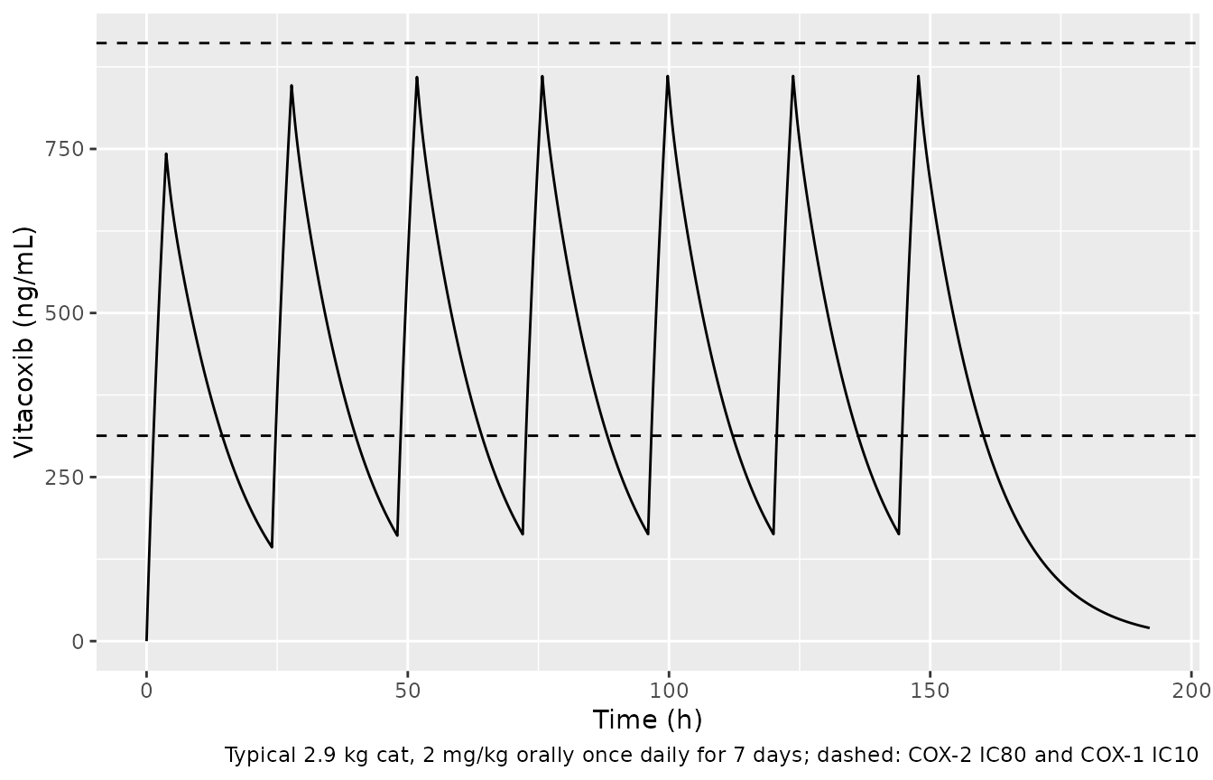
acc <- max(sim_md$Cc[sim_md$time >= 144]) / max(sim_md$Cc[sim_md$time <= 24])
acc
#> [1] 1.159356
stopifnot(acc > 1, acc < 1.3)

With an effective half-life under a day at 0.319 L/h, accumulation over seven daily doses is modest.

Assumptions and deviations

Clearance unit. Table 2 and the Abstract give CL as 0.11 L/h (110 ml/h). The model carries 0.11 as L/h/kg and multiplies by body weight. Two independent checks support this: the deterministic replication of the paper’s Figure 6 above (RMSE about 1 h against more than 20 h for the printed unit, best-fitting multiplier about 2.9 = the mean weight), and the companion NCA clearance of 95 ml/kg/h from the same i.v. data. The paper’s derived statements that inherit the printed unit – a half-life of about 21 h (0.693 x VSS / CL), a clearance of 1.8 ml/min and an extraction ratio below 0.01 – are therefore not reproduced by this model; with the per-kg clearance the same formula gives about 7.4 h for a 2.9 kg cat. The paper does not state whether the per-kg clearance was scaled by each cat’s weight or by a fixed weight; linear weight scaling is used here, and at the cohort mean weight both readings are identical. Q (0.52 L/h) is kept as printed: Figure 6 is insensitive to it.
Weight covariate on V1. Equation 2 prints log(V1i) = log(V1pop) + beta x WT0i + eta. WT0 is taken to be the log-normalised weight log(WT / 2.9) that Methods says was evaluated; the raw-weight reading would give a typical V1 of 9.4 L, contradicting the reported VSS of 3.42 L and the Figure 6 dose thresholds. The centring value 2.9 kg is the reported cohort mean (the paper’s “weighted mean bodyweight” is not printed separately).
Random effects. Table 2 reports only between-occasion variability (as CV%), states that most variability was within-subject, and prints no separate between-animal magnitudes. The tabulated values are encoded as one random effect per parameter, to be redrawn for each dosing occasion; simulating a new occasion of the same animal as a new id reproduces this. For log-normal parameters omega^2 = log(1 + CV^2); for the logit-normal F and Fr the percentage is taken as the logit-scale SD. The Ka and Q values (10.0%) are the random effects the Results say were set to 0.1 and are fixed.
Feeding and sex. Feeding status (Study 3) and sex were screened and not retained; they are listed in covariatesDataExcluded.
Pharmacodynamic targets. The COX-1 IC10/IC20 and COX-2 IC80/IC90 values (911.3, 1467.8, 313.0, 556.5 ng/mL) are in-vitro whole-blood assay results used only as simulation thresholds; no PD model was fitted, so none is encoded.