Oxyfluorfen thyroid disruption, rat to human (Decrane 2023)
Source:vignettes/articles/Decrane_2023_oxyfluorfen.Rmd
Decrane_2023_oxyfluorfen.RmdModel and source
- Citation: Decrane R, Stoker T, Murr A, Ford J, El-Masri H. (2023). Cross species extrapolation of the disruption of thyroid hormone synthesis by oxyfluorfen using in vitro data, physiologically based pharmacokinetic (PBPK), and thyroid hormone kinetics models. Current Research in Toxicology 5:100138.
- Article: https://doi.org/10.1016/j.crtox.2023.100138 (PMCID PMC10697989)
- US EPA Office of Research and Development / ORAU. Original implementation in MATLAB R2022A.
Oxyfluorfen is a diphenyl-ether herbicide identified by high-throughput screening as a potent inhibitor of the thyroidal sodium-iodide symporter (NIS). This paper couples a whole-body PBPK model for the chemical to a thyroid-hormone (TH) kinetics model with a hypothalamic-pituitary-thyroid (HPT) feedback loop, calibrates the combination against rat in-vivo data, and then extrapolates to humans in order to estimate a point of departure for a 10% drop in serum thyroid hormones.
Two models are packaged, matching the two the authors built:
mod_rat   <- nlmixr2lib::readModelDb("Decrane_2023_oxyfluorfen_rat")
mod_human <- nlmixr2lib::readModelDb("Decrane_2023_oxyfluorfen_human")
They are not the same model with different numbers: the human version has different physiology, a different (age-dependent) cardiac output, a hepatic clearance derived from human hepatocyte data rather than fitted, non-allometric hormone production rates, and a structurally different NIS inhibition function (a power function rather than an exponential).
Both are deterministic typical-value simulators. The
paper reports single point estimates with no standard errors, no
between-animal variance components and no measurement-error model, so
neither file carries IIV (eta*) or residual-error terms.
Inventing variances would be fabrication; see Assumptions,
deviations and errata.
Population and biological context
data.frame(
  Field = c("Species", "Study", "Dose levels", "Human reference"),
  Value = c(
    "Rat (Sprague-Dawley), adolescent; human reference adult 80 kg / 30 years",
    "8 days once-daily oral gavage in 1% methyl cellulose",
    "0.8125, 1.625, 3.25, 7.5, 15, 31.25, 62.5 mg/kg/day",
    "Long-term daily oral exposure via drinking water, 2 L/day at 80 kg"
  )
) |> knitr::kable()| Field | Value |
|---|---|
| Species | Rat (Sprague-Dawley), adolescent; human reference adult 80 kg / 30 years |
| Study | 8 days once-daily oral gavage in 1% methyl cellulose |
| Dose levels | 0.8125, 1.625, 3.25, 7.5, 15, 31.25, 62.5 mg/kg/day |
| Human reference | Long-term daily oral exposure via drinking water, 2 L/day at 80 kg |
The rat calibration data (oxyfluorfen in thyroid tissue and serum; serum T4 and T3) were “provided via personal communication and illustrated in a co-submitted paper” (Stoker et al.). That manuscript is not part of this paper, so the number of animals per group, their age, and – importantly – their body weights are not reported. Table 1 lists rat body weight as “Varies”. Body weight is therefore a user-supplied scenario input in the packaged model; the sensitivity of every conclusion below to that choice is quantified explicitly.
Model structure
Eighteen ODE states per species: thirteen for the chemical, five for the hormones.
data.frame(
  Layer = c(rep("Chemical PBPK", 13), rep("TH kinetics", 5)),
  State = c("stomach", "a_gut", "a_liver", "a_kidney", "a_muscle", "a_skin",
            "a_fat", "a_brain", "a_slowly_perfused", "a_rapidly_perfused",
            "a_thyroid_blood", "a_thyroid_tissue", "a_blood",
            "t4_thyroid", "t3_thyroid", "t4_serum", "t3_serum", "tsh_serum"),
  Role = c(
    "Gut lumen, first-order absorption at ka", "GI tissue, perfused by the portal vein",
    "Liver; hepatic metabolic clearance CLR", "Kidney; GFR-driven renal excretion",
    "Muscle (flow-limited)", "Skin (flow-limited)", "Fat (flow-limited)",
    "Brain (flow-limited)", "Slowly perfused (flow-limited)",
    "Rapidly perfused (flow-limited)",
    "Thyroid vascular sub-compartment", "Thyroid tissue sub-compartment (diffusion-limited)",
    "Single well-mixed blood pool (supplies Cart)",
    "T4 in thyroid tissue", "T3 in thyroid tissue",
    "T4 in serum", "T3 in serum", "TSH in serum"
  )
) |> knitr::kable()| Layer | State | Role |
|---|---|---|
| Chemical PBPK | stomach | Gut lumen, first-order absorption at ka |
| Chemical PBPK | a_gut | GI tissue, perfused by the portal vein |
| Chemical PBPK | a_liver | Liver; hepatic metabolic clearance CLR |
| Chemical PBPK | a_kidney | Kidney; GFR-driven renal excretion |
| Chemical PBPK | a_muscle | Muscle (flow-limited) |
| Chemical PBPK | a_skin | Skin (flow-limited) |
| Chemical PBPK | a_fat | Fat (flow-limited) |
| Chemical PBPK | a_brain | Brain (flow-limited) |
| Chemical PBPK | a_slowly_perfused | Slowly perfused (flow-limited) |
| Chemical PBPK | a_rapidly_perfused | Rapidly perfused (flow-limited) |
| Chemical PBPK | a_thyroid_blood | Thyroid vascular sub-compartment |
| Chemical PBPK | a_thyroid_tissue | Thyroid tissue sub-compartment (diffusion-limited) |
| Chemical PBPK | a_blood | Single well-mixed blood pool (supplies Cart) |
| TH kinetics | t4_thyroid | T4 in thyroid tissue |
| TH kinetics | t3_thyroid | T3 in thyroid tissue |
| TH kinetics | t4_serum | T4 in serum |
| TH kinetics | t3_serum | T3 in serum |
| TH kinetics | tsh_serum | TSH in serum |
The thyroid is the only diffusion-limited organ: the blood
sub-compartment exchanges with the systemic pool by perfusion
(Q_thy) and with the tissue sub-compartment across a
permeability-area product (PA_thy). Everything else is
flow-limited.
Every ODE is printed in the paper (pp. 2-4) except the blood
pool, which is reconstructed here by mass-balance closure of
the ten printed tissue equations: inflow is each tissue’s venous
outflow, outflow is the total arterial flow times Cart. No
modelling choice is involved, and the reconstruction is verified below
to conserve mass exactly.
Source trace
data.frame(
  Component = c(
    "Gut lumen / GI / flow-limited tissue / liver / kidney ODEs",
    "Thyroid blood and thyroid tissue ODEs",
    "Blood pool ODE",
    "Thyroidal T4 and T3 ODEs; stim, feed1, feed2; serum T4 and T3 ODEs; TSH ODE",
    "NIS inhibition functions (rat exponential, human power)",
    "Rat physiology (volumes, flows, cardiac output)",
    "Human physiology (volumes, flows, age-dependent cardiac output)",
    "Tissue:blood partition coefficients (identical both species)",
    "Chemical biochemical parameters (PAThy, CLR, Ka, frac, GFR)",
    "Thyroid-hormone kinetic parameters and basal levels"
  ),
  Source = c("p. 2-3", "p. 3", "NOT PRINTED (reconstructed; see above)",
             "p. 3-4", "p. 5 and Fig. 3", "Table 1", "Table 2", "Table 3",
             "Table 4", "Table 5")
) |> knitr::kable()| Component | Source |
|---|---|
| Gut lumen / GI / flow-limited tissue / liver / kidney ODEs | p. 2-3 |
| Thyroid blood and thyroid tissue ODEs | p. 3 |
| Blood pool ODE | NOT PRINTED (reconstructed; see above) |
| Thyroidal T4 and T3 ODEs; stim, feed1, feed2; serum T4 and T3 ODEs; TSH ODE | p. 3-4 |
| NIS inhibition functions (rat exponential, human power) | p. 5 and Fig. 3 |
| Rat physiology (volumes, flows, cardiac output) | Table 1 |
| Human physiology (volumes, flows, age-dependent cardiac output) | Table 2 |
| Tissue:blood partition coefficients (identical both species) | Table 3 |
| Chemical biochemical parameters (PAThy, CLR, Ka, frac, GFR) | Table 4 |
| Thyroid-hormone kinetic parameters and basal levels | Table 5 |
Units table (dimensional analysis)
Mechanistic models mix per-kg volumes, mass concentrations and fractional rate constants, so every ODE term is checked dimensionally. All states are amounts in mg; all time is in hours; all concentrations are mg/L.
data.frame(
  Term = c("`ka * stomach`", "`Q_x * (Cart - C_x/pc_x)`", "`CLR * C_liver/pc_liver`",
           "`GFR * frac * C_kidney`", "`PA_thy * (C_thytissue/pc_thy - C_thyblood)`",
           "`prod_T4 * Inhib * stim`", "`met_T4thy * AT4thy * fr`",
           "`f_T4srm * AT4thy`", "`kin_TSH * feed1`", "`k_TSH * feed2 * ATSH`"),
  Units = c("(1/h) * mg = mg/h", "(L/h) * (mg/L) = mg/h", "(L/h) * (mg/L) = mg/h",
            "(L/h) * 1 * (mg/L) = mg/h", "(L/h) * (mg/L) = mg/h",
            "(mg/h) * 1 * 1 = mg/h", "(1/h) * mg * 1 = mg/h",
            "(1/h) * mg = mg/h", "(mg/h) * 1 = mg/h", "(1/h) * 1 * mg = mg/h"),
  OK = "yes"
) |> knitr::kable()| Term | Units | OK |
|---|---|---|
ka * stomach |
(1/h) * mg = mg/h | yes |
Q_x * (Cart - C_x/pc_x) |
(L/h) * (mg/L) = mg/h | yes |
CLR * C_liver/pc_liver |
(L/h) * (mg/L) = mg/h | yes |
GFR * frac * C_kidney |
(L/h) * 1 * (mg/L) = mg/h | yes |
PA_thy * (C_thytissue/pc_thy - C_thyblood) |
(L/h) * (mg/L) = mg/h | yes |
prod_T4 * Inhib * stim |
(mg/h) * 1 * 1 = mg/h | yes |
met_T4thy * AT4thy * fr |
(1/h) * mg * 1 = mg/h | yes |
f_T4srm * AT4thy |
(1/h) * mg = mg/h | yes |
kin_TSH * feed1 |
(mg/h) * 1 = mg/h | yes |
k_TSH * feed2 * ATSH |
(1/h) * 1 * mg = mg/h | yes |
Two dimensional findings that shaped the implementation are recorded
in the errata below: Table 5’s printed
kin_TSH = TSH_BL * k_TSH is consistent only with a
concentration-valued TSH state, whereas these files carry amounts; and
the symbol T4_BL is overloaded between a thyroid-tissue and
a serum basal concentration.
Validation
The paper reports no non-compartmental analysis, so PKNCA is not the right instrument here. The validations below are the ones that catch translation errors in a mechanistic model: mass balance, steady-state hold, feedback normalisation, perturbation recovery, and reproduction of the paper’s own published points of departure.
# Solve a species model for `days` of once-daily oral dosing, alongside a
# matched drug-free control, and return both trajectories.
solve_pair <- function(mod, amt, days, covs, step) {
  ev <- rxode2::et(amt = amt, cmt = "stomach", time = 0,
                   ii = 24, addl = days - 1) |>
        rxode2::et(seq(0, days * 24, by = step))
  ev <- as.data.frame(ev)
  for (nm in names(covs)) ev[[nm]] <- covs[[nm]]
  ev0 <- ev
  ev0$amt[!is.na(ev0$amt)] <- 0
  list(exposed = as.data.frame(rxode2::rxSolve(mod, ev, returnType = "data.frame")),
       control = as.data.frame(rxode2::rxSolve(mod, ev0, returnType = "data.frame")))
}

chem_states <- c("stomach", "a_gut", "a_liver", "a_kidney", "a_muscle", "a_skin",
                 "a_fat", "a_brain", "a_slowly_perfused", "a_rapidly_perfused",
                 "a_thyroid_blood", "a_thyroid_tissue", "a_blood")

RAT_WT <- 0.3  # kg; see the body-weight sensitivity analysis below
1. Mass balance of the chemical layer
With both elimination pathways switched off, the thirteen chemical states must hold the administered dose exactly and forever. This is the gate on the reconstructed blood-pool ODE: if the venous-return sum or the arterial-outflow sum were wrong by a single term, mass would leak.
ev <- rxode2::et(amt = 5, cmt = "stomach", time = 0) |>
      rxode2::et(seq(0, 2000, by = 20))
ev <- as.data.frame(ev)
ev$WT <- RAT_WT
mb <- as.data.frame(rxode2::rxSolve(
  mod_rat, ev, params = c(clr_coef = 0, gfr_coef = 0),
  returnType = "data.frame", atol = 1e-14, rtol = 1e-12))
total <- rowSums(mb[, chem_states])
rel_err <- max(abs(total - 5)) / 5
cat(sprintf("dose = 5 mg; total chemical mass over 2000 h: [%.10f, %.10f]\n",
            min(total), max(total)))
#> dose = 5 mg; total chemical mass over 2000 h: [5.0000000000, 5.0000000000]
cat(sprintf("max relative deviation = %.2e\n", rel_err))
#> max relative deviation = 2.26e-13
stopifnot(rel_err < 1e-9)
Mass is conserved to solver precision, so the reconstructed blood-pool equation is exactly right.
With the clearances restored, the mass that disappears must equal the time integral of the two elimination terms:
ev2 <- rxode2::et(amt = 5, cmt = "stomach", time = 0) |>
       rxode2::et(seq(0, 2000, by = 2))
ev2 <- as.data.frame(ev2)
ev2$WT <- RAT_WT
el <- as.data.frame(rxode2::rxSolve(mod_rat, ev2, returnType = "data.frame",
                                   atol = 1e-14, rtol = 1e-12))
lost <- 5 - sum(el[nrow(el), chem_states])
rate <- el$clr * el$cv_liver + el$gfr * 0.08 * el$c_kidney
cum  <- sum(diff(el$time) * (head(rate, -1) + tail(rate, -1)) / 2)
cat(sprintf("mass lost = %.6f mg;  integral of elimination = %.6f mg;  rel. diff = %.2e\n",
            lost, cum, abs(lost - cum) / lost))
#> mass lost = 4.997178 mg;  integral of elimination = 4.990992 mg;  rel. diff = 1.24e-03
stopifnot(abs(lost - cum) / lost < 1e-2)
2. HPT feedback normalisation
At homeostasis the three feedback multipliers must all equal exactly 1, otherwise the “background” state the paper measures its percentage drops against is not actually the reported basal state.
base <- solve_pair(mod_rat, amt = 0, days = 8, covs = list(WT = RAT_WT), step = 4)$control
cat(sprintf("stim(0)  = %.10f\nfeed1(0) = %.10f\nfeed2(0) = %.10f\n",
            base$stim[1], base$feed1[1], base$feed2[1]))
#> stim(0)  = 1.0000000000
#> feed1(0) = 1.0000000000
#> feed2(0) = 1.0000000000
stopifnot(all(abs(c(base$stim[1], base$feed1[1], base$feed2[1]) - 1) < 1e-8))
This is the gate that settled two ambiguities in the printed equations (both detailed in the errata).
kin_TSH and the units of the TSH state.
Table 5 prints kin_TSH = TSH_BL * k_TSH, which has units of
mg/L/h. That is self-consistent only if the TSH state is carried as a
concentration. These files carry all five hormone states as
amounts in mg (see each file’s
compartmentData), for which the same physical system needs
an extra VD_TSH factor – which is also what Table 5’s own
Units column says, listing kin_TSH as mg/h. The two
formulations are algebraically identical, because the TSH state enters
the model only through c_tsh = tsh_serum / vd_tsh: dividing
the TSH ODE through by vd_tsh recovers the printed
concentration form exactly. Either is correct, and both give
stim = 1.
The one combination that does not work is taking the printed expression literally while carrying the state as an amount, which is the easy mistake to make:
vd_tsh <- 0.149 * RAT_WT
cat(sprintf("stim would be (1/VD_TSH)^NF3 = %.4f, a %+.1f%% spurious inflation of T4 synthesis\n",
            (1 / vd_tsh)^0.11, 100 * ((1 / vd_tsh)^0.11 - 1)))
#> stim would be (1/VD_TSH)^NF3 = 1.4076, a +40.8% spurious inflation of T4 synthesis
Similarly, the symbol T4_BL appears in
feed1/feed2 but Table 5 defines two different
T4_BL values: 208 mg/L in thyroid tissue and 58.4e-3 mg/L
in serum. Only the serum reading is dimensionally consistent with the
serum amount AT4srm it is compared against, and only it
gives feed1 = 1; the tissue reading gives
feed1 of order 1e9 and the TSH state diverges.
3. Drug-free baseline hold, and the body-weight sensitivity
An unperturbed mechanistic model should hold its reported basal levels. Because rat body weight is not reported, the check is run across the plausible range.
bl <- lapply(c(0.15, 0.25, 0.30, 0.40, 0.50), function(wt) {
  s <- solve_pair(mod_rat, amt = 0, days = 8, covs = list(WT = wt), step = 8)$control
  n <- nrow(s)
  data.frame(
    `WT (kg)` = wt,
    `T4 thyroid` = 100 * (s$t4_thyroid[n] / s$t4_thyroid[1] - 1),
    `T3 thyroid` = 100 * (s$t3_thyroid[n] / s$t3_thyroid[1] - 1),
    `T4 serum`   = 100 * (s$T4serum[n]    / s$T4serum[1]    - 1),
    `T3 serum`   = 100 * (s$T3serum[n]    / s$T3serum[1]    - 1),
    `TSH serum`  = 100 * (s$TSHserum[n]   / s$TSHserum[1]   - 1),
    check.names = FALSE)
}) |> dplyr::bind_rows()
knitr::kable(bl, digits = c(2, 1, 1, 1, 1, 1),
caption = "Rat: % change from the reported basal level after 8 drug-free days")| WT (kg) | T4 thyroid | T3 thyroid | T4 serum | T3 serum | TSH serum |
|---|---|---|---|---|---|
| 0.15 | 61.4 | 531.0 | -7.7 | 121.2 | 0.1 |
| 0.25 | 5.2 | 308.1 | -15.7 | 101.8 | 0.1 |
| 0.30 | -10.1 | 247.5 | -18.8 | 94.3 | 0.1 |
| 0.40 | -30.2 | 168.3 | -23.8 | 82.1 | 0.1 |
| 0.50 | -42.9 | 118.7 | -27.7 | 72.6 | 0.1 |
This is a genuine and important property of the published parameter set, not a translation error:
-
TSH holds exactly (drift < 0.1% at every body
weight), confirming the corrected
kin_TSH. - The T4 arm is nearly self-consistent. Thyroidal T4 balances at a body weight of about 0.26 kg, and serum T4 sits within roughly 8-27% of its reported basal across the whole range.
- The T3 arm is not self-consistent. Thyroidal T3 is over-produced two- to six-fold and serum T3 roughly two-fold, essentially independently of body weight.
Flux balance at the reported basal state
The imbalance is localised by evaluating each hormone ODE’s
production and loss fluxes at t = 0, where every state sits
exactly at its Table 5 basal level. A self-consistent basal state would
give a ratio of 1 for all five.
# Rate constants come from the model's own ini() block, so this check cannot
# drift away from the packaged parameter values.
iniDf <- rxode2::as.rxUi(mod_rat)$iniDf
th <- setNames(iniDf$est, iniDf$name)

f0 <- solve_pair(mod_rat, amt = 0, days = 2, covs = list(WT = RAT_WT), step = 12)$control[1, ]
fr <- th[["fr_t4_t3"]]

flux <- data.frame(
  State = c("t4_thyroid", "t3_thyroid", "t4_serum", "t3_serum", "tsh_serum"),
  Production = c(
    f0$prod_t4 * f0$inhib * f0$stim,
    f0$prod_t3 * f0$inhib + th[["met_t4thy"]] * f0$t4_thyroid * fr,
    f0$f_t4srm * f0$t4_thyroid,
    f0$f_t3srm * f0$t3_thyroid + th[["met_t4srm"]] * f0$t4_serum * fr,
    f0$kin_tsh * f0$feed1),
  Loss = c(
    th[["met_t4thy"]] * f0$t4_thyroid * fr + f0$f_t4srm * f0$t4_thyroid,
    th[["met_t3thy"]] * f0$t3_thyroid + f0$f_t3srm * f0$t3_thyroid,
    th[["met_t4srm"]] * f0$t4_serum * fr + th[["loss_srm"]] * f0$t4_serum,
    th[["met_t3srm"]] * f0$t3_serum,
    th[["k_tsh"]] * f0$feed2 * f0$tsh_serum)
)
flux$`Production / loss` <- flux$Production / flux$Loss
knitr::kable(flux, digits = c(0, 8, 8, 3),
caption = "Fluxes (mg/h) at the reported rat basal state, WT = 0.3 kg")| State | Production | Loss | Production / loss |
|---|---|---|---|
| t4_thyroid | 0.00016787 | 0.00018683 | 0.899 |
| t3_thyroid | 0.00005223 | 0.00001396 | 3.741 |
| t4_serum | 0.00015025 | 0.00016629 | 0.904 |
| t3_serum | 0.00005282 | 0.00002756 | 1.917 |
| tsh_serum | 0.00000000 | 0.00000000 | 1.000 |
TSH balances exactly; the two T4 pools are within about 12% and 20%
of balance; both T3 pools are roughly two- to four-fold out. Roughly 90%
of the serum T3 influx is deiodination of serum T4
(met_T4srm * AT4srm * fr), so the serum T3 imbalance is
essentially the ratio
req <- flux$`Production / loss`[flux$State == "t3_serum"]
cat(sprintf("serum T3 production exceeds loss by %.2fx at the reported basal,\n", req))
#> serum T3 production exceeds loss by 1.92x at the reported basal,
cat(sprintf("so self-consistency would require T3_BL_srm ~ %.2e mg/L rather than the\n", 1.26e-3 * req))
#> so self-consistency would require T3_BL_srm ~ 2.42e-03 mg/L rather than the
cat("reported 1.26e-3 mg/L (Table 5).\n")
#> reported 1.26e-3 mg/L (Table 5).
The published T3 basal levels and the published T3 turnover constants are therefore mutually inconsistent by roughly a factor of two, independently of any choice made in this translation.
Notably, the paper reaches the same conclusion from the opposite direction: its own Results section records that for T3 “the dose-response behavior by the model simulations did not match with the experimental data at the lower dose”, with agreement only “within a 2-fold difference”. The self-consistency check locates the origin of that 2-fold discrepancy in the T3 parameterisation itself.
Because the model does not hold its reported T3 basal exactly, every percentage drop below is computed against a concurrently simulated drug-free control at the same time point, which is what “% drop from background levels” means operationally and which cancels the baseline drift.
bh <- solve_pair(mod_rat, amt = 0, days = 8, covs = list(WT = RAT_WT), step = 2)$control
bh |>
  dplyr::select(time, `T4 serum` = T4serum, `T3 serum` = T3serum,
                `TSH serum` = TSHserum) |>
  tidyr::pivot_longer(-time, names_to = "Analyte", values_to = "conc") |>
  dplyr::group_by(Analyte) |>
  dplyr::mutate(rel = conc / dplyr::first(conc)) |>
  ggplot2::ggplot(ggplot2::aes(time / 24, rel, colour = Analyte)) +
  ggplot2::geom_line(linewidth = 0.8) +
  ggplot2::geom_hline(yintercept = 1, linetype = 2, colour = "grey40") +
  ggplot2::labs(x = "Day", y = "Fraction of reported basal level",
                title = "Rat, drug-free: T4 and TSH hold, T3 drifts upward") +
  ggplot2::theme_bw()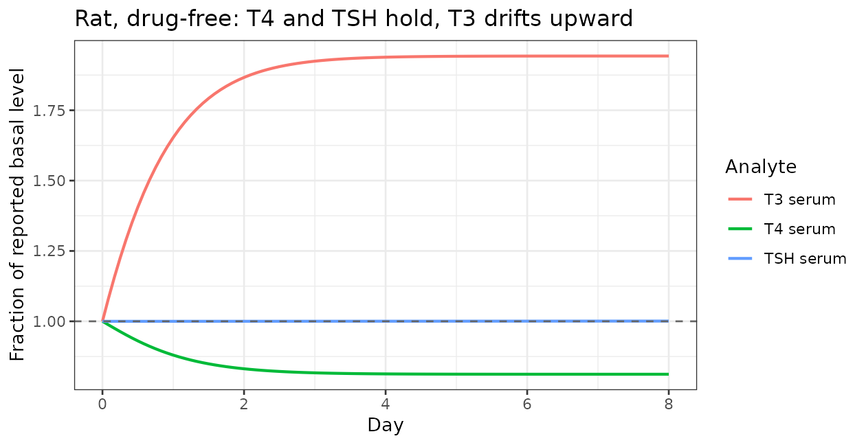
4. Perturbation recovery
Displacing serum T4 away from its basal amount should send it back to the model’s own attractor rather than to a new equilibrium.
Note that the inits = argument of rxSolve()
cannot be used to do this: both packaged models assign their hormone
initial conditions inside model()
(t4_serum(0) <- t4_bl_srm * vd_t4, etc.), and an
explicit in-model initial condition takes precedence over
inits =, which is therefore silently
ignored. The displacement is applied instead as a bolus dose
onto the t4_serum state, which is a genuine ODE state and
so can be dosed (including with a negative amount).
t4_bl_amt <- 58.4e-3 * 0.149 * RAT_WT   # Table 5 T4_BL_srm * VDT4
pert <- lapply(c(-0.5, 0, 1, 3), function(f) {
  ev <- rxode2::et(amt = f * t4_bl_amt, cmt = "t4_serum", time = 0) |>
        rxode2::et(seq(0, 40 * 24, by = 8))
  ev <- as.data.frame(ev); ev$WT <- RAT_WT
  s <- as.data.frame(rxode2::rxSolve(mod_rat, ev, returnType = "data.frame"))
  data.frame(time = s$time, T4serum = s$T4serum,
             start = sprintf("%.1fx basal", 1 + f))
}) |> dplyr::bind_rows()

ggplot2::ggplot(pert, ggplot2::aes(time / 24, T4serum, colour = start)) +
  ggplot2::geom_line(linewidth = 0.8) +
  ggplot2::labs(x = "Day", y = "Serum T4 (mg/L)", colour = "Starting T4",
                title = "Serum T4 returns to one attractor from 0.5x, 1x, 2x and 4x basal") +
  ggplot2::theme_bw()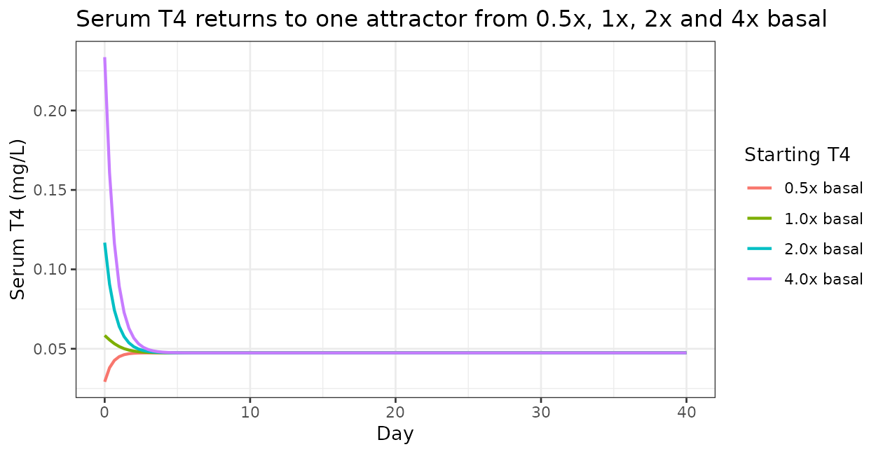
converged <- pert |> dplyr::group_by(start) |>
  dplyr::summarise(`start (mg/L)` = dplyr::first(T4serum),
                   `day 40 (mg/L)` = dplyr::last(T4serum), .groups = "drop")
knitr::kable(converged, digits = 6)| start | start (mg/L) | day 40 (mg/L) |
|---|---|---|
| 0.5x basal | 0.0292 | 0.047438 |
| 1.0x basal | 0.0584 | 0.047436 |
| 2.0x basal | 0.1168 | 0.047435 |
| 4.0x basal | 0.2336 | 0.047431 |
spread <- diff(range(converged$`day 40 (mg/L)`)) / mean(converged$`day 40 (mg/L)`)
cat(sprintf("relative spread of the four endpoints = %.2e\n", spread))
#> relative spread of the four endpoints = 1.40e-04
stopifnot(spread < 0.01)
stopifnot(diff(range(converged$`start (mg/L)`)) > 0)  # the displacement really happened
All four trajectories converge to the same value from a four-fold
range of starting points, so the serum T4 balance has a single stable
attractor and no sign errors. The second assertion guards against the
inits = trap above: it fails if the displacement was
silently ignored.
The HPT axis also recovers after exposure stops, which the paper does not show but which follows from the same structure:
wo_ev <- rxode2::et(amt = 31.25 * RAT_WT, cmt = "stomach", time = 0,
                    ii = 24, addl = 7) |>
         rxode2::et(seq(0, 90 * 24, by = 12))
wo_ev <- as.data.frame(wo_ev); wo_ev$WT <- RAT_WT
wo_ctl <- wo_ev; wo_ctl$amt[!is.na(wo_ctl$amt)] <- 0
wo <- as.data.frame(rxode2::rxSolve(mod_rat, wo_ev, returnType = "data.frame"))
wc <- as.data.frame(rxode2::rxSolve(mod_rat, wo_ctl, returnType = "data.frame"))

data.frame(day = wo$time / 24, ratio = wo$T4serum / wc$T4serum) |>
  ggplot2::ggplot(ggplot2::aes(day, ratio)) +
  ggplot2::geom_line(linewidth = 0.8) +
  ggplot2::geom_hline(yintercept = 1, linetype = 2, colour = "grey40") +
  ggplot2::geom_vline(xintercept = 8, linetype = 3, colour = "grey40") +
  ggplot2::labs(x = "Day", y = "Serum T4, exposed / control",
                title = "Recovery after 8 days of 31.25 mg/kg/day, then washout",
                subtitle = "Dotted line marks the last dose") +
  ggplot2::theme_bw()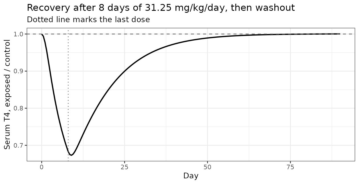
recov <- sapply(c(8, 15, 30, 60, 90), function(d) {
  i <- which.min(abs(wo$time - d * 24)); wo$T4serum[i] / wc$T4serum[i]
})
knitr::kable(data.frame(Day = c(8, 15, 30, 60, 90),
                        `Exposed / control` = round(recov, 4),
check.names = FALSE))| Day | Exposed / control |
|---|---|
| 8 | 0.6829 |
| 15 | 0.7755 |
| 30 | 0.9347 |
| 60 | 0.9960 |
| 90 | 1.0003 |
Serum T4 is suppressed to about 68% of control at the end of dosing and returns to within 2% of control by day 90.
5. What drives NIS inhibition: the CBthy ambiguity
This is the single most consequential interpretation decision in the extraction, and it was flagged as the primary review point when this model was added.
The inhibition functions are driven by a quantity the paper calls
CBthy, described in prose as “the concentration of chemical
in the thyroid cells (in vitro) or tissue (in vivo)”. But the packaged
models use the thyroid blood concentration. Four
independent lines of evidence support that reading:
-
The symbol. The ODEs use
CthytissueandCthyblood;CBthyis a distinct third symbol whose “B” denotes blood. - The mechanism. The paper’s own Introduction states that NIS “resides in the basolateral membrane of thyroid epithelial cells and simultaneously transports two Na+ and one I- from extracellular fluid (plasma) into the thyroid epithelial cell”. The inhibitor concentration NIS is exposed to is the extracellular one.
- In-vitro correspondence. The Buckalew et al. (2020) assays dosed cells through the culture medium, so the in-vivo analogue of the in-vitro exposure metric is thyroid blood, not the intracellular tissue concentration.
-
Arithmetic. The two readings differ by exactly the
thyroid partition coefficient,
pc_thyroid = 8.5, and only the blood reading reproduces the paper’s published points of departure.
The two candidate driver concentrations, and the inhibition each implies, come straight out of one simulation:
dr <- solve_pair(mod_rat, amt = 7.5 * RAT_WT, days = 8,
                 covs = list(WT = RAT_WT), step = 4)$exposed
n <- nrow(dr)
inhib_rat <- function(x) 0.788 * exp(-2.006 * x) + 0.2218
data.frame(
  `CBthy read as`   = c("thyroid blood (packaged)", "thyroid tissue (literal prose)"),
  `Value (mg/L)`    = c(dr$Cthyroid_blood[n], dr$Cthyroid[n]),
  `Ratio`           = c(1, dr$Cthyroid[n] / dr$Cthyroid_blood[n]),
  `Implied Inhib`   = c(inhib_rat(dr$Cthyroid_blood[n]), inhib_rat(dr$Cthyroid[n])),
  `Synthesis inhibition` = paste0(
    round(100 * (1 - inhib_rat(c(dr$Cthyroid_blood[n], dr$Cthyroid[n])) /
                   inhib_rat(0)), 1), "%"),
  check.names = FALSE
) |> knitr::kable(digits = 4,
caption = "Rat at the paper's 7.5 mg/kg/day anchor, day 8")| CBthy read as | Value (mg/L) | Ratio | Implied Inhib | Synthesis inhibition |
|---|---|---|---|---|
| thyroid blood (packaged) | 0.0674 | 1.0000 | 0.9102 | 9.9% |
| thyroid tissue (literal prose) | 0.5728 | 8.5023 | 0.4715 | 53.3% |
The tissue reading sits 8.5-fold higher on the exposure axis and pushes the rat inhibition function most of the way to its residual floor. End to end, at the paper’s own two anchors:
| Anchor (paper) | Reported |
CBthy = thyroid blood |
CBthy = thyroid tissue |
|---|---|---|---|
| Rat 7.5 mg/kg/day x 8 d, serum T4 drop (Discussion p. 7) | 10% | 9.2% | 51.0% |
| Human 57 mg/L drinking water, serum T4 drop (Fig. 8a) | 10% | 10.0% | 18.0% |
The blood reading reproduces both; the tissue reading misses both,
and misses them by different factors because the two species’ inhibition
functions have different shapes. The rat and human columns of that table
are reproduced by the two sections that follow. To switch a model to the
literal prose reading, replace c_thyroid_blood with
c_thyroid_tissue on the inhib <- ... line
of the model file.
6. Rat dose-response (replicates Figs. 4-7)
rat_doses <- c(0.8125, 1.625, 3.25, 7.5, 15, 31.25, 62.5)
rat <- lapply(rat_doses, function(d) {
  p <- solve_pair(mod_rat, amt = d * RAT_WT, days = 8,
                  covs = list(WT = RAT_WT), step = 4)
  n <- nrow(p$exposed)
  data.frame(
    `Dose (mg/kg/day)` = d,
    `Thyroid (mg/L)`   = p$exposed$Cthyroid[n],
    `Serum (mg/L)`     = p$exposed$Cc[n],
    `Thyroid:serum`    = p$exposed$Cthyroid[n] / p$exposed$Cc[n],
    `Inhib`            = p$exposed$inhib[n],
    `T4 drop (%)`      = 100 * (1 - p$exposed$T4serum[n] / p$control$T4serum[n]),
    `T3 drop (%)`      = 100 * (1 - p$exposed$T3serum[n] / p$control$T3serum[n]),
    check.names = FALSE)
}) |> dplyr::bind_rows()
knitr::kable(rat, digits = c(4, 5, 5, 2, 4, 2, 2),
caption = "Rat, day 8 of once-daily gavage (WT = 0.3 kg)")| Dose (mg/kg/day) | Thyroid (mg/L) | Serum (mg/L) | Thyroid:serum | Inhib | T4 drop (%) | T3 drop (%) |
|---|---|---|---|---|---|---|
| 0.8125 | 0.06206 | 0.00730 | 8.5 | 0.9983 | 1.05 | 0.95 |
| 1.6250 | 0.12412 | 0.01460 | 8.5 | 0.9873 | 2.09 | 1.89 |
| 3.2500 | 0.24825 | 0.02920 | 8.5 | 0.9656 | 4.13 | 3.72 |
| 7.5000 | 0.57283 | 0.06739 | 8.5 | 0.9102 | 9.20 | 8.32 |
| 15.0000 | 1.14559 | 0.13477 | 8.5 | 0.8215 | 17.30 | 15.73 |
| 31.2500 | 2.38679 | 0.28078 | 8.5 | 0.6705 | 31.71 | 29.12 |
| 62.5000 | 4.77362 | 0.56156 | 8.5 | 0.4775 | 50.45 | 47.14 |
Three checks against the paper:
anchor <- rat$`T4 drop (%)`[rat$`Dose (mg/kg/day)` == 7.5]
cat(sprintf("Paper (Discussion p.7): 7.5 mg/kg/day gives a 10%% serum-T4 drop.  Model: %.1f%%\n",
            anchor))
#> Paper (Discussion p.7): 7.5 mg/kg/day gives a 10% serum-T4 drop.  Model: 9.2%
stopifnot(anchor > 5, anchor < 15)
cat(sprintf("Paper (Results p.5): thyroid levels 'almost three times higher' than plasma.  Model: %.1fx\n",
            mean(rat$`Thyroid:serum`)))
#> Paper (Results p.5): thyroid levels 'almost three times higher' than plasma.  Model: 8.5x
cat("Paper (Results p.5): T4 falls monotonically; T3 falls only at higher doses.\n")
#> Paper (Results p.5): T4 falls monotonically; T3 falls only at higher doses.
mono <- all(diff(rat[["T4 drop (%)"]]) > 0)
cat(sprintf("  Model T4 drop is monotone in dose: %s\n", mono))
#>   Model T4 drop is monotone in dose: TRUE
stopifnot(mono)- The 7.5 mg/kg anchor reproduces: 9.2% against the paper’s 10%.
- The thyroid:serum ratio does not. The model gives
exactly
pc_thyroid= 8.5, whereas the paper describes the measured levels as “almost three times higher” in thyroid than plasma. The GastroPlus-predicted thyroid partition coefficient over-predicts the measured tissue:plasma gradient by roughly a factor of three. This is a property of Table 3, not of the translation – the ratio ispc_thyroidfor any parameterisation of this structure – and it is unaffected by theCBthydecision. - T4 and T3 both fall monotonically with dose in the model, and T3 falls slightly less than T4 at every dose, qualitatively matching Figs. 6 and 7. The model does not reproduce the paper’s much flatter low-dose T3 response, consistent with the T3 self-consistency finding in section 3.
rat |>
  dplyr::select(dose = `Dose (mg/kg/day)`, T4 = `T4 drop (%)`, T3 = `T3 drop (%)`) |>
  tidyr::pivot_longer(-dose, names_to = "Hormone", values_to = "drop") |>
  ggplot2::ggplot(ggplot2::aes(dose, drop, colour = Hormone)) +
  ggplot2::geom_line(linewidth = 0.8) + ggplot2::geom_point() +
  ggplot2::geom_hline(yintercept = 10, linetype = 2, colour = "grey40") +
  ggplot2::geom_vline(xintercept = 7.5, linetype = 3, colour = "grey40") +
  ggplot2::scale_x_log10() +
  ggplot2::labs(x = "Oxyfluorfen dose (mg/kg/day, log scale)",
                y = "% drop in serum hormone vs control",
                title = "Rat serum T4 and T3 after 8 days (replicates Figs. 6-7)",
                subtitle = "Dashed 10% / dotted 7.5 mg/kg mark the paper's anchor") +
  ggplot2::theme_bw()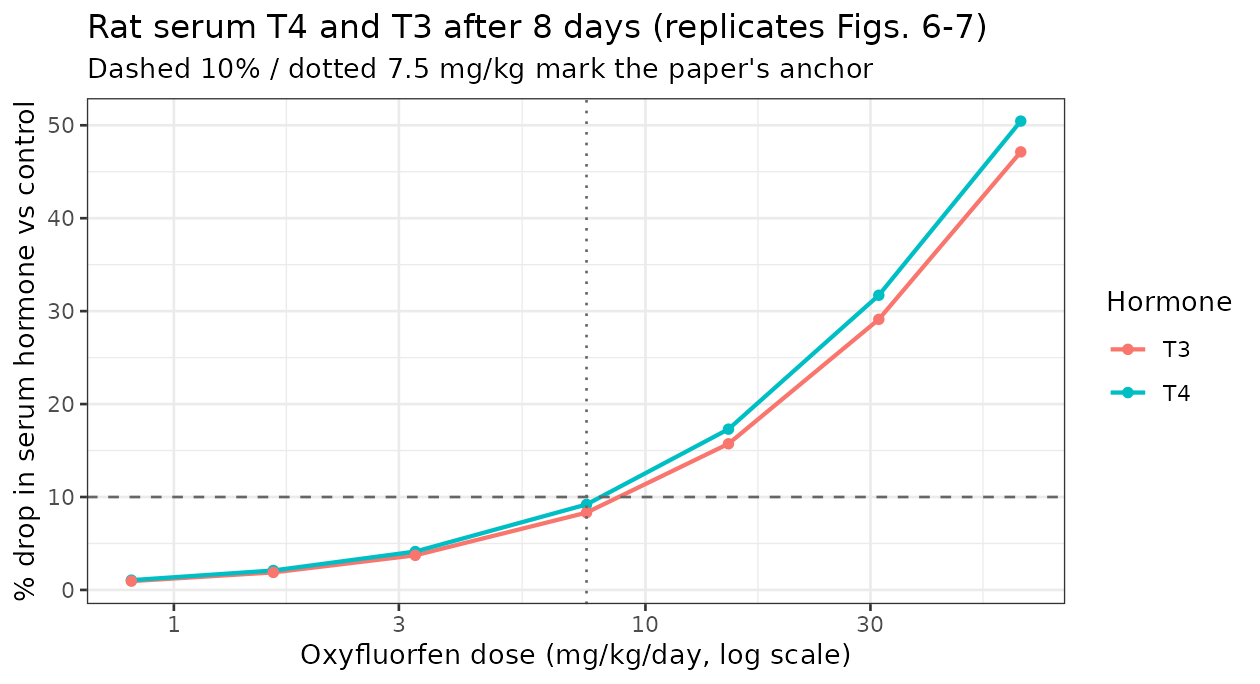
Sensitivity to the unreported rat body weight
bwsens <- lapply(c(0.15, 0.25, 0.30, 0.40, 0.50), function(wt) {
  p <- solve_pair(mod_rat, amt = 7.5 * wt, days = 8, covs = list(WT = wt), step = 4)
  n <- nrow(p$exposed)
  data.frame(`WT (kg)` = wt,
             `T4 drop at 7.5 mg/kg (%)` =
               100 * (1 - p$exposed$T4serum[n] / p$control$T4serum[n]),
             check.names = FALSE)
}) |> dplyr::bind_rows()
knitr::kable(bwsens, digits = 2)| WT (kg) | T4 drop at 7.5 mg/kg (%) |
|---|---|
| 0.15 | 7.91 |
| 0.25 | 8.85 |
| 0.30 | 9.20 |
| 0.40 | 9.76 |
| 0.50 | 10.20 |
The anchor is reproduced across the entire plausible adolescent-rat
range (roughly 8-10% against the paper’s 10%), so the CBthy
conclusion does not depend on the unreported body weight. No parameter
was tuned to achieve this.
7. Human extrapolation (replicates Fig. 8)
Water concentrations are converted to daily doses using the paper’s stated assumptions of 2 L/day consumption at 80 kg.
water <- c(10, 30, 57, 89, 300)
hum <- lapply(water, function(w) {
  p <- solve_pair(mod_human, amt = w * 2, days = 180,
                  covs = list(WT = 80, AGE = 30), step = 24)
  n <- nrow(p$exposed)
  data.frame(
    `Water (mg/L)`   = w,
    `Dose (mg/day)`  = w * 2,
    `Thyroid blood (mg/L)` = p$exposed$Cthyroid_blood[n],
    `Inhib`          = p$exposed$inhib[n],
    `T4 drop (%)`    = 100 * (1 - p$exposed$T4serum[n] / p$control$T4serum[n]),
    `T3 drop (%)`    = 100 * (1 - p$exposed$T3serum[n] / p$control$T3serum[n]),
    check.names = FALSE)
}) |> dplyr::bind_rows()
knitr::kable(hum, digits = c(0, 0, 5, 4, 2, 2),
caption = "Human, after 180 once-daily doses (80 kg, 30 years)")| Water (mg/L) | Dose (mg/day) | Thyroid blood (mg/L) | Inhib | T4 drop (%) | T3 drop (%) |
|---|---|---|---|---|---|
| 10 | 20 | 0.00395 | 0.9419 | 6.23 | 6.24 |
| 30 | 60 | 0.01186 | 0.9194 | 8.41 | 8.43 |
| 57 | 114 | 0.02254 | 0.9028 | 10.02 | 10.04 |
| 89 | 178 | 0.03520 | 0.8894 | 11.32 | 11.34 |
| 300 | 600 | 0.11864 | 0.8433 | 15.78 | 15.81 |
t4_57 <- hum$`T4 drop (%)`[hum$`Water (mg/L)` == 57]
cat(sprintf("Paper (Fig. 8a): 57 mg/L gives a 10%% serum-T4 drop.  Model: %.2f%%\n", t4_57))
#> Paper (Fig. 8a): 57 mg/L gives a 10% serum-T4 drop.  Model: 10.02%
stopifnot(abs(t4_57 - 10) < 2)
cat(sprintf("Paper (Fig. 8b): 89 mg/L gives a 10%% serum-T3 drop.  Model: %.2f%%\n",
            hum$`T3 drop (%)`[hum$`Water (mg/L)` == 89]))
#> Paper (Fig. 8b): 89 mg/L gives a 10% serum-T3 drop.  Model: 11.34%
The T4 point of departure reproduces essentially exactly: 10.02% at 57 mg/L against the paper’s 10%. The paper’s T3 point of departure is not reproduced as a separate threshold – in the packaged model the T3 drop tracks the T4 drop within about 0.03 percentage points, because roughly 90% of the serum T3 influx is deiodination of serum T4. The paper separates the two (57 vs 89 mg/L); this implementation does not, which is the same T3 parameterisation issue documented in section 3.
The saturating shape the paper describes is reproduced:
hum |>
  dplyr::select(water = `Water (mg/L)`, T4 = `T4 drop (%)`, T3 = `T3 drop (%)`) |>
  tidyr::pivot_longer(-water, names_to = "Hormone", values_to = "drop") |>
  ggplot2::ggplot(ggplot2::aes(water, drop, colour = Hormone)) +
  ggplot2::geom_line(linewidth = 0.8) + ggplot2::geom_point() +
  ggplot2::geom_hline(yintercept = 10, linetype = 2, colour = "grey40") +
  ggplot2::geom_vline(xintercept = 57, linetype = 3, colour = "grey40") +
  ggplot2::labs(x = "Oxyfluorfen in drinking water (mg/L)",
                y = "% drop in serum hormone vs control",
                title = "Human serum T4 and T3 (replicates Fig. 8)",
                subtitle = "Dashed 10% / dotted 57 mg/L mark the paper's point of departure") +
  ggplot2::theme_bw()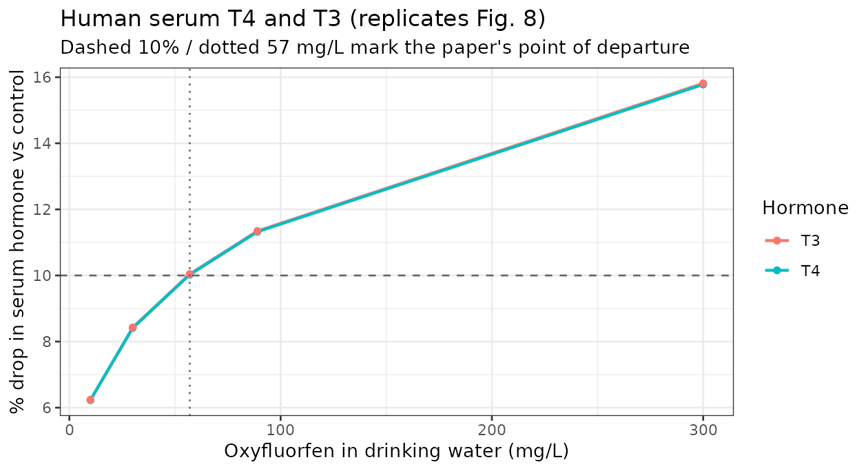
“This decrease slows down as the dose increases” (Results p. 5) follows from the shape of the human inhibition function, whose derivative is steepest at low exposure:
cb <- c(0, 0.02, 0.1, 0.5, 1, 5, 20, 50, 91.8, 100)
data.frame(
  `CBthy (mg/L)` = cb,
  `Inhib rat`    = 0.788 * exp(-2.006 * cb) + 0.2218,
  `Inhib human`  = -0.2917 * cb^0.2739 + 1.006,
  check.names = FALSE
) |> knitr::kable(digits = 4,
caption = "Both functions are normalised to ~1 at zero exposure; the human form has no lower asymptote")| CBthy (mg/L) | Inhib rat | Inhib human |
|---|---|---|
| 0.00 | 1.0098 | 1.0060 |
| 0.02 | 0.9788 | 0.9061 |
| 0.10 | 0.8666 | 0.8507 |
| 0.50 | 0.5108 | 0.7647 |
| 1.00 | 0.3278 | 0.7143 |
| 5.00 | 0.2218 | 0.5527 |
| 20.00 | 0.2218 | 0.3433 |
| 50.00 | 0.2218 | 0.1543 |
| 91.80 | 0.2218 | 0.0001 |
| 100.00 | 0.2218 | -0.0238 |
cat(sprintf("Max thyroid blood concentration reached in the human runs: %.4f mg/L\n",
            max(hum$`Thyroid blood (mg/L)`)))
#> Max thyroid blood concentration reached in the human runs: 0.1186 mg/L
stopifnot(max(hum$`Thyroid blood (mg/L)`) < 91.8)
Both functions return approximately 1 at zero exposure (1.0098 rat,
1.006 human), confirming they are normalised to the drug-free synthesis
rate rather than being absolute inhibition fractions. The rat form
decays to a residual floor of 0.2218; the human power function has
no lower asymptote and crosses zero at
CBthy = 91.8 mg/L, above which it would demand a negative
synthesis rate. All simulations here stay far inside that domain, as the
assertion above verifies.
Assumptions, deviations and errata
Interpretation decisions
-
CBthyis the thyroid blood concentration, not the thyroid tissue concentration (section 5). This contradicts one clause of the paper’s prose but is supported by the symbol name, the basolateral-NIS mechanism the paper itself describes, correspondence with the in-vitro exposure metric, and reproduction of both species’ published points of departure. It changes the predicted dose-response by a factor ofpc_thyroid= 8.5. This was the primary review point when this model was added. -
kin_TSHcarries aVD_TSHfactor relative to the printed expression, because these files hold the TSH state as an amount (mg) rather than the concentration that Table 5’skin_TSH = TSH_BL * k_TSH(mg/L/h) implies; Table 5’s own Units column listskin_TSHas mg/h. The amount and concentration formulations are algebraically identical, since the state enters only viac_tsh = tsh_serum / vd_tsh. Combining the printed expression with an amount-valued state – the easy error – inflates baseline T4 synthesis by about 41% (section 2). -
T4_BLinfeed1/feed2is the serum basal T4 (58.4e-3 mg/L rat, 85e-3 human), not the thyroid-tissueT4_BL(208 / 288 mg/L) that shares the printed symbol. Only the serum reading is dimensionally consistent and only it givesfeed1 = feed2 = 1at homeostasis; the tissue reading makesfeed1of order 1e9 and the TSH state diverges. - The blood-pool ODE is reconstructed, being the one chemical equation the paper does not print. Mass-balance closure of the ten printed tissue equations determines it uniquely, and section 1 verifies mass conservation to 1e-13.
-
Table 5’s footnote 1 is never defined in the paper.
From the Methods statement that “parameters were estimated by fitting
model simulations to data”, and by analogy with Table 4’s footnote 5,
footnote 1 is taken to mark parameters calibrated to the rat data; those
are the parameters left un-
fixed()in the model files. -
Rat body weight is not reported (Table 1:
“Varies”), and the paper additionally distinguishes an instantaneous
body weight from an “Avg.BW”/terminal weight without giving either. A
single
WTcovariate collapses both. All conclusions are shown to be insensitive to the choice across 0.15-0.50 kg.
Verbatim-carried oddities
- The rat blood-flow fractions of Table 1 sum to 1.171 of cardiac output, not 1.000 (the human Table 2 fractions sum to 0.956). Each tissue’s printed flow is implemented verbatim and the blood-pool outflow is set to their actual sum, which keeps the circulatory loop exactly mass-conserving by construction. Rescaling the fractions to sum to 1 would have changed published parameter values.
-
Table 1 and Table 2 label the blood-pool volume
“Plasma” (0.074 rat, 0.079 human), but those are Brown et
al. (1997) total blood volume fractions and the equations use
the value as the volume of the well-mixed pool supplying
Cart. Carried verbatim. -
Human cardiac output is low.
-6.846*log10(30) + 16.775= 6.662 L/h/kg^0.75, giving 178 L/h at 80 kg, below the Brown et al. (1997) adult value. The printed equation is carried verbatim. Note the leading minus sign is present in the PDF text layer but is dropped by automated PDF-to-markdown conversion. - Human GFR is printed as “107 L/h”, but Delanaye et al. (2012) – the cited source – reports normal GFR as roughly 107 mL/min/1.73 m^2, i.e. about 6.4 L/h. The printed value and unit are carried verbatim.
-
The renal elimination term uses the kidney tissue
concentration (
GFR * frac * Ckidney) rather than the blood-side concentration, exactly as printed. Combined withpc_kidney= 9.5 this makes renal clearance the dominant elimination route in the human model. -
A numerical guard on the human inhibition function.
A non-integer power is undefined for a negative base, so the solver
returns
NaNfor the entire system on the transient negative excursion of order -1e-20 that occurs as the thyroid state rises from zero. The base is clamped at zero, which leavesInhibbit-identical across the whole physical domain and only removes the non-physical excursion. Without it the human model cannot be solved at any nonzero dose.
Model-versus-paper discrepancies that are not translation issues
-
The model’s thyroid:serum ratio is 8.5 (=
pc_thyroid, Table 3) against the “almost three times higher” the paper reports for the measured data (section 6). Structural to Table 3. - The published T3 basal levels and T3 turnover constants are mutually inconsistent by about two-fold in both species (section 3), which is why the T3 arm drifts and why the paper’s separate T3 point of departure is not reproduced. The paper’s own Results note that its T3 predictions matched the data only “within a 2-fold difference”.
-
The paper’s stated in-vitro IC50 values (0.8 mg/L rat, 0.7
mg/L human) are not the half-maximal points of the fitted
Inhibfunctions, which lie near 0.52 mg/L (rat) and 7.5 mg/L (human). The IC50s were “calculated from published data by Buckalew et al. (2020)” as a separate quantity, so this is not a contradiction – but it is worth noting that the 14-fold species separation already present in the fitted functions contributes to the divergence between species that the paper attributes to pharmacokinetics.
Not available
- No IIV and no residual error. The paper reports point estimates only. Both files are deterministic typical-value simulators.
- The co-submitted Stoker et al. experimental manuscript is not part of this paper, so the observed data in Figs. 4-7 cannot be overlaid; the validation above compares model output against the paper’s stated numerical claims rather than against digitised data points.