Desipramine whole-body PBPK (Samant 2017)
Source:vignettes/articles/Samant_2017_desipramine_pbpk.Rmd
Samant_2017_desipramine_pbpk.RmdModel and source
- Citation: Samant TS, Lukacova V, Schmidt S. Development and Qualification of Physiologically Based Pharmacokinetic Models for Drugs With Atypical Distribution Behavior: A Desipramine Case Study. CPT Pharmacometrics Syst Pharmacol. 2017;6(5):315-321. doi:10.1002/psp4.12180. Physiology, partition coefficients and observed data are taken from the deposited GastroPlus project in Supporting Information file PSP4-6-315-s003.zip (physiology file HumAmeMal34.4YO_83.4kg.pbk; compound database Desipramine-reordered.mdb, table PBPKParams, record ‘IV Adult 12.5 mg Male’); clearance, Vss and plasma unbound fraction by age are from the Supplementary Table (PSP4-6-315-s001.docx).
- Description: PBPK (whole-body, perfusion-limited, GastroPlus v8.6). Intravenous desipramine in a human reference adult: 13 perfusion-limited tissues (lung, adipose, muscle, liver, spleen, heart, brain, kidney, skin, reproductive organs, red marrow, yellow marrow, rest of body) between arterial and venous blood pools, with the gut and spleen draining into the liver. The paper’s atypical distribution (Vss about 15 L/kg from phospholipid binding and lysosomal trapping) is carried by the deposited tissue:plasma partition coefficients, which the authors computed with a raised blood:plasma ratio before reverting it to 1.03. Renal clearance is fu x GFR. Hepatic clearance is anchored to the paper’s own simulated total plasma clearance (Supplementary Table) and converted to a well-stirred intrinsic clearance inside model(); the paper’s CYP2D6 in vitro scaling and ontogeny are not reproduced. The oral ACAT arm (enterocyte trapping) is not included. Default values are the 34.4-year, 83.4 kg male used for the 12.5 mg IV model-building arm; the deposited physiology and Kp sets for other ages and sexes are substituted through ini() (see the vignette). Deterministic typical-value model with no between-subject or residual variability.
- Article: https://doi.org/10.1002/psp4.12180
- Supporting information (open access, Europe PMC): https://www.ebi.ac.uk/europepmc/webservices/rest/PMC5697013/supplementaryFiles
Samant, Lukacova and Schmidt built a GastroPlus v8.6 whole-body PBPK model for desipramine, a tricyclic base whose steady-state volume of distribution (10-50 L/kg) is far larger than the standard tissue-partitioning methods predict. They captured it by computing the tissue:plasma partition coefficients (Kp) with an inflated blood:plasma ratio (2.4 in males, 2.7 in females) as a surrogate for phospholipid binding and lysosomal trapping, then reverting the blood:plasma ratio to its predicted 1.03 for simulation. The adult intravenous model was then extended to oral dosing (enterocyte trapping, fraction unbound in enterocytes 0.55%) and scaled to children.
What this port contains
The main text does not print the PBPK equations or the physiology, but the supporting information deposits the GastroPlus project itself: one physiology file per simulated individual (17 tissues with volumes, blood flows and connectivity, plus GFR and hematocrit), the compound database with the per-tissue Kp of every simulated scenario, the digitised observed data of the four adult arms, and a Supplementary Table of simulated clearance (CL), Vss and plasma unbound fraction by age and sex. Those deposited files fully specify the intravenous distribution model, which is what this port implements.
Two parts of the paper are not reproduced:
-
Hepatic metabolism is not predicted from CYP2D6
kinetics. CYP2D6 accounts for about 97% of desipramine
clearance. The printed in vitro Vmax and Km (68 pmol/min/mg, 6.1 uM)
scale to a whole-liver intrinsic clearance roughly an order of magnitude
below the one the published profiles require, and the GastroPlus enzyme
normalisation and CYP2D6 ontogeny that close that gap are built into the
platform and not documented. The maintainers therefore anchored total
plasma clearance to the paper’s own Supplementary Table (CL in mL/h/kg
by age and sex), subtracted renal clearance (fu x GFR), and converted
the remainder to a well-stirred hepatic intrinsic clearance inside
model(). The clearance versus age curve (paper Figure 4) is therefore an input of this model, not a prediction. - The oral arm is not included. The deposited physiology files carry the gut only as a reference to GastroPlus’s built-in ACAT intestinal model, with no segment volumes, transit times, pH profile or absorption scale factors, so the oral profiles (Figure 3) and the enterocyte-trapping parameter cannot be ported.
Population
No individual data were fitted. The adult intravenous model was developed against the published mean profile after a 12.5 mg IV bolus in healthy volunteers (Ciraulo 1988, paper reference 22) and externally qualified against a 50 mg IV bolus (Brosen and Gram 1988, reference 23). Each arm is simulated in one GastroPlus PEAR reference individual whose physiology file is deposited: an 83.4 kg, 34.4-year male for 12.5 mg and a 70.1 kg, 30-year female for 50 mg. The paediatric extrapolation uses deposited reference individuals of both sexes at birth (term), 0.5, 1, 2.5, 5, 10 and 15 years, and adults at 22, 27 and 34.5 years.
str(readModelDb("Samant_2017_desipramine_pbpk")()$population)
#> List of 9
#>  $ species      : chr "human"
#>  $ n_subjects   : int NA
#>  $ n_studies    : int 4
#>  $ age_range    : chr "Adults 22-42 years (simulated reference individuals); paediatric extrapolation 0-15 years"
#>  $ weight_range : chr "70-85.1 kg adults; 3.1-69.4 kg paediatric reference individuals"
#>  $ disease_state: chr "Healthy volunteers (literature mean profiles)"
#>  $ dose_range   : chr "12.5 and 50 mg IV bolus (this model); 50 and 100 mg oral (paper, not included)"
#>  $ regions      : chr "Not reported"
#>  $ notes        : chr "No individual data were fitted. The model was built against the published mean profile after 12.5 mg IV in norm"| __truncated__
Source trace
Every ini() value carries an in-file comment naming its
deposited source.
| Element | Value (reference male) | Source |
|---|---|---|
| Model structure: 13 perfusion-limited tissues between arterial and venous blood; gut and spleen drain to the liver | – | Methods (‘all tissues are perfusion-limited’); physiology file tissue list and ConnectIn/ConnectOut topology |
| IV bolus enters venous blood | – | physiology file Settings InfusionKey = 4 (Venous
Return) |
bp |
1.03 | Table 1; Methods (‘reverted back to the predicted value of 1.03’);
database RatioBloodPlasma
|
fup |
0.178 | Supplementary Table, Fup column (GastroPlus adjusted value; Table 1 lists the unadjusted 0.19) |
cl_kg |
508 mL/h/kg | Supplementary Table, 34.5 years, males |
| Renal clearance = fup x GFR | – | Methods (’renal clearance was estimated as fu*GFR’); database
KidneyCLEstMethod = Fup*GFR
|
gfr |
1.942 mL/s | physiology file GlomerularFiltrationRate
|
kp_* (13 tissues) |
5.9-66.0 | compound database PBPKParams, record ‘IV Adult 12.5 mg
Male’ |
vol_* (15 volumes) |
mL | physiology file HumAmeMal34.4YO_83.4kg.pbk,
Volume of each tissue |
perf_* (13 flows) |
mL/s | same file, TissuePerfusion of each tissue; hepatic
artery and ACAT gut give the two non-splenic liver inflows |
wt |
83.4 kg | physiology file Weight; observed-data file ‘Body Wt
[kg] = 83.4’ |
| Observed profiles | – | deposited IV_Adult_12.5_mg_Male.ipd and
IV_Adult_50_mg_Female.ipd
|
The deposited flows were checked when the table below was transcribed: in every physiology file the arterial-side flows sum to the cardiac output (lung perfusion) and the hepatic artery, gut and spleen flows sum to the liver perfusion, both to better than 1 part in a million.
Deposited individuals
The table holds, for each simulated individual, the deposited
physiology (in the units of the physiology files: mL and mL/s), the
deposited Kp set for that individual’s scenario, and the Supplementary
Table CL, Vss and plasma unbound fraction for that age and sex.
M34.5_ap is the reference male with the un-optimised Kp set
(record ‘Desipramine AP6.5’, computed with the predicted blood:plasma
ratio 1.03) used for the paper’s Figure 2c. F30 is the 50
mg IV individual; the Supplementary Table has no 30-year row, so its
clearance is interpolated linearly in age between the 27- and 34.5-year
female values.
subjects <- read.csv(text = "
id,age,sexf,wt,hct,fup,cl_kg,vss_kg,gfr,vol_arterial,vol_venous,vol_lung,vol_adipose,vol_muscle,vol_liver,vol_spleen,vol_heart,vol_brain,vol_kidney,vol_skin,vol_reproductive_organs,vol_red_marrow,vol_yellow_marrow,vol_other,perf_hepatic_artery,perf_gut,perf_adipose,perf_muscle,perf_spleen,perf_heart,perf_brain,perf_kidney,perf_skin,perf_reproductive_organs,perf_red_marrow,perf_yellow_marrow,perf_other,kp_lung,kp_adipose,kp_muscle,kp_liver,kp_spleen,kp_heart,kp_brain,kp_kidney,kp_skin,kp_reproductive_organs,kp_red_marrow,kp_yellow_marrow,kp_other
M0,0.00273973,0,3.19,0.532597,0.239,140,15.7,0.0472222,77.6599,155.32,55.6148,1040.36,510.979,106.783,10.1503,18.4297,392.786,25.3555,136.558,1.89917,41.2309,0.508462,477.26,1.17639,1.30415,0.586765,0.432288,0.286309,0.379485,5.65022,2.6319,0.462248,0.011249,0.348896,0.00043,0.403762,50.612,5.83297,20.1944,59.1545,41.3028,29.2951,5.761,65.0923,17.3642,65.0819,9.30824,5.83297,41.3117
F0,0.00273973,1,3.09,0.532597,0.239,163,17.7,0.0472222,74.8586,149.717,52.8644,1008.98,502.884,105.117,8.81702,18.4297,358.985,23.2955,129.73,1.23806,39.1693,0.282297,483.694,1.35009,1.3563,0.853598,0.42544,0.258647,0.499038,5.26524,2.11581,0.548887,0.007333,0.331451,0.000239,0.409205,59.2536,6.71702,23.5758,69.2326,48.331,34.2678,6.64505,76.2093,20.2816,76.1989,10.789,6.71702,48.3399
M0.5,0.5,0,7.94,0.356969,0.198,817,10.2,0.394967,156.217,312.434,105.854,4041.64,1325.57,211.654,20.0066,36.8931,738.082,48.0328,216.548,2.28303,102.83,8.34999,330.086,2.23638,1.80623,1.87532,0.921272,0.463714,0.624231,8.72487,4.09696,0.602221,0.011112,0.714978,0.005803,0.229409,51.0871,5.84415,20.3072,59.6735,41.6643,29.5507,5.75617,65.7012,17.4918,65.6933,9.2978,5.84415,41.6654
F0.5,0.5,1,7.39,0.356969,0.198,947,10.3,0.394967,135.781,271.562,101.877,4114.46,1188.14,202.18,16.88,36.8931,660.641,43.0438,205.721,1.99321,97.7886,7.56896,60.9808,2.40079,1.87844,2.85955,0.825758,0.406892,0.820909,7.9627,3.21249,0.715292,0.009701,0.679924,0.00526,0.042382,59.7287,6.7282,23.6887,69.7517,48.6925,34.5235,6.64022,76.8181,20.4092,76.8102,10.7786,6.7282,48.6936
M1,1,0,10.25,0.388042,0.195,886,10.4,0.501695,216.499,432.997,142.322,4604.87,1827.45,300.572,27.0165,48.7059,987.817,63.8842,240.95,2.6416,182.471,27.0165,488.48,3.15345,2.21282,1.9847,1.18053,0.582043,0.765998,10.8541,5.06493,0.622855,0.011951,1.17931,0.017453,0.315558,51.1379,5.85061,20.3226,59.7243,41.7043,29.5848,5.78143,65.7649,17.5138,65.7576,9.31399,5.85061,41.7014
F1,1,1,9.5,0.388042,0.195,1029,11,0.501695,172.902,345.804,140.647,4608.46,1687.61,286.147,23.2483,48.7059,883.074,57.7002,228.902,2.616,173.41,25.3894,211.762,3.34257,2.30129,2.97707,1.0902,0.520902,1.00734,9.89308,4.00278,0.739812,0.011835,1.12075,0.016402,0.136798,59.7795,6.73466,23.7041,69.8025,48.7325,34.5576,6.66548,76.8818,20.4311,76.8745,10.7948,6.73466,48.7296
M2.5,2.5,0,15.04,0.40983,0.192,847,12.3,0.749125,369.502,739.005,196.468,4659.18,3658.38,455.514,40.92,67.8476,1276.4,88.3207,345.514,3.47378,337.311,114.679,1234.13,3.83605,2.45586,1.55151,1.82919,0.682013,0.825502,10.8494,5.41697,0.691027,0.012158,1.68655,0.05734,0.617064,51.1668,5.87132,20.3349,59.7543,41.7349,29.6101,5.82452,65.8085,17.5278,65.8023,9.3729,5.87132,41.7255
F2.5,2.5,1,14.21,0.40983,0.192,985,18.7,0.749125,272.728,545.457,185.626,2728.95,3456.49,444.205,38.4568,61.4683,1154.69,89.058,326.446,3.81206,325.587,112.074,2912.91,4.32386,2.41314,1.36448,1.72824,0.666572,0.983494,10.0077,4.77948,0.816115,0.013342,1.62794,0.056037,1.45645,59.8084,6.75537,23.7164,69.8325,48.7631,34.5829,6.70857,76.9255,20.4452,76.9192,10.8537,6.75537,48.7537
M5,5,0,21.46,0.4175,0.189,733,11.4,1.02133,603.45,1206.9,280.333,5498.66,5220,564.981,52.8502,90.885,1457.05,112.729,493,3.914,764.706,492.221,1324.88,4.26484,3.50417,1.83106,2.61,0.880854,1.1058,12.3849,6.91399,0.986,0.013699,3.82353,0.24611,0.662439,51.2007,5.89774,20.3507,59.8094,41.7757,29.6411,5.85833,65.8634,17.5463,65.8581,9.51229,5.89774,41.7621
F5,5,1,20.93,0.4175,0.189,846,17,1.02133,483.679,967.358,273.41,3229.23,5091.08,565.556,45.5865,84.1273,1375.85,110.998,480.824,4.46,762.681,499.727,3484.04,5.08164,3.55433,1.61461,2.54554,0.790152,1.34604,11.9245,5.95694,1.20206,0.01561,3.8134,0.249864,1.74202,59.8423,6.78179,23.7322,69.8876,48.8039,34.6138,6.74238,76.9803,20.4637,76.975,10.9931,6.78179,48.7903
M10,10,0,42.4,0.43284,0.182,513,16.2,1.5751,876.583,1753.17,553.874,10698.5,10313.5,793.579,72.512,142.176,1681.61,159.585,974.054,5.041,1006.1,1249.01,8200.74,4.01772,6.92342,3.5626,5.15676,1.20856,1.72986,14.2937,9.78786,1.94811,0.017643,5.03052,0.624505,4.10037,51.2649,5.93081,20.3805,59.9138,41.853,29.6995,5.88694,65.9638,17.5881,65.9596,9.94302,5.93081,41.8381
F10,10,1,44.14,0.43284,0.182,574,17.3,1.5751,766.68,1533.36,576.604,13835.3,10736.8,823.617,69.2403,140.283,1580.23,147.193,1014.03,7.4265,1027.81,1287.19,6847.77,5.03123,7.49585,6.91764,5.36838,1.20014,2.24453,13.6958,7.89938,2.53507,0.025993,5.13908,0.643594,3.42388,59.9065,6.81486,23.762,69.9919,48.8812,34.6723,6.77099,77.0808,20.5054,77.0765,11.4238,6.81486,48.8663
M15,15,0,69.41,0.44818,0.178,509,17.4,1.89654,2046.41,4092.81,906.707,17015.3,16883.5,1328.8,119.479,230.052,1793.58,231.299,1594.55,26.653,1181.78,2283.21,15033.8,7.01866,11.3338,5.66609,8.44176,1.99135,2.79905,15.2454,14.1863,3.18911,0.093285,5.90889,1.14161,7.51688,51.2988,5.94626,20.4025,59.9827,41.9064,29.742,5.90323,66.0229,17.6252,66.0192,10.5776,5.94626,41.8931
F15,15,1,63.37,0.44818,0.178,575,16.4,1.89654,1390.86,2781.71,827.806,23425.4,15414.3,1213.16,114.291,211.73,1622.12,221.3,1455.8,25.058,1125.09,2142.07,7737.61,7.47732,10.7615,11.7127,7.70716,1.98101,3.38768,14.0589,11.8765,3.63949,0.087703,5.62547,1.07104,3.8688,59.9404,6.83031,23.784,70.0609,48.9346,34.7148,6.78728,77.1398,20.5426,77.1361,12.0584,6.83031,48.9213
M22,22,0,82.48,0.45,0.178,503,16.1,2.05137,2192.28,4384.57,1077.44,25322.2,20062.7,1579.01,170.292,312.039,1751.7,285.714,1894.81,31.0125,1159.58,3223.24,14939.8,7.86835,13.468,8.4323,10.0314,2.83826,3.79658,14.8894,17.5237,3.78962,0.108544,5.79792,1.61162,7.4699,51.289,5.95113,20.4146,60.0074,41.9188,29.7683,5.92563,66.019,17.6216,66.019,9.35359,5.95113,41.9189
F22,22,1,70.67,0.45,0.178,569,15.8,2.05137,1534.43,3068.86,923.167,28128.8,17190,1352.92,144.903,246.172,1621.03,260,1623.5,102.796,1095.67,2887.75,7334.79,8.03629,12.0012,14.0644,8.595,2.51161,3.93875,14.0495,13.9534,4.05875,0.359788,5.47835,1.44387,3.66739,59.9306,6.83518,23.7961,70.0856,48.947,34.7411,6.80968,77.1359,20.539,77.1359,10.8344,6.83518,48.9471
M27,27,0,85.12,0.45,0.178,502,15.8,2.03822,2220,4439.99,1111.93,27827.9,20704.9,1629.55,175.473,321.743,1744.16,285.714,1955.46,32.0051,1180.76,3282.1,14194.2,8.12469,13.8991,9.2667,10.3524,2.92461,3.91464,14.8253,17.5237,3.91092,0.112018,5.90379,1.64105,7.09708,51.289,5.95113,20.4146,60.0074,41.9188,29.7683,5.92563,66.019,17.6216,66.019,9.35359,5.95113,41.9189
F27,27,1,74.04,0.45,0.178,567,15.1,2.03822,1599.18,3198.37,967.189,31439.2,18009.7,1417.43,150.375,251.897,1608.71,260,1700.92,216.518,1122.46,2958.35,6102.3,8.44443,12.5735,15.7196,9.00487,2.60645,4.03035,13.9427,13.9534,4.2523,0.757813,5.6123,1.47918,3.05115,59.9306,6.83518,23.7961,70.0856,48.947,34.7411,6.80968,77.1359,20.539,77.1359,10.8344,6.83518,48.9471
M34.5,34.4,0,83.4,0.45,0.178,508,15.1,1.94246,2133.86,4267.73,1089.46,29799.5,20286.5,1596.62,162.687,317.459,1650.49,271.923,1915.95,31.3584,1142.18,3174.87,11903.4,8.21551,13.7877,10.0467,10.2695,2.74525,3.9106,14.2038,16.8854,3.87958,0.11112,5.78198,1.60719,6.02577,51.289,5.95113,20.4146,60.0074,41.9188,29.7683,5.92563,66.019,17.6216,66.019,9.35359,5.95113,41.9189
F34.5,34.5,1,76.76,0.45,0.178,573,14.4,1.94097,1651.34,3302.69,1002.72,34858.6,18671.4,1469.5,150.473,260.484,1600.67,260,1763.41,514.408,1143.91,3014.88,4217.76,8.84872,13.0354,17.4293,9.33568,2.60814,4.16775,13.873,13.9534,4.40851,1.80043,5.71954,1.50744,2.10888,59.9586,6.72607,23.7849,70.0827,48.949,34.7329,6.74811,77.1532,20.5198,77.1532,10.7679,6.72607,48.949
F30,30,1,70.1,0.45,0.178,NA,NA,2.0051,1511.46,3022.93,915.721,30581.4,17051.4,1342,141.146,237.952,1496.15,242.303,1610.41,293.738,1054.8,2780.03,5043.68,8.15886,12.116,15.5625,8.67725,2.48998,3.87493,13.1976,13.2348,4.09759,1.04636,5.36777,1.41473,2.56667,59.9306,6.83518,23.7961,70.0856,48.947,34.7411,6.80968,77.1359,20.539,77.1359,10.8344,6.83518,48.9471
M34.5_ap,34.4,0,83.4,0.45,0.178,508,15.1,1.94246,2133.86,4267.73,1089.46,29799.5,20286.5,1596.62,162.687,317.459,1650.49,271.923,1915.95,31.3584,1142.18,3174.87,11903.4,8.21551,13.7877,10.0467,10.2695,2.74525,3.9106,14.2038,16.8854,3.87958,0.11112,5.78198,1.60719,6.02577,12.1264,1.6065,4.99861,14.2355,9.99773,7.14848,1.69599,15.5947,4.30074,15.5947,2.42058,1.6065,9.99775
", stringsAsFactors = FALSE)

# Supplementary Table has no 30-year row: interpolate CL linearly in age
# between the 27- and 34.5-year female values.
f27 <- subjects[subjects$id == "F27", ]
f345 <- subjects[subjects$id == "F34.5", ]
subjects$cl_kg[subjects$id == "F30"] <-
  f27$cl_kg + (30 - f27$age) / (f345$age - f27$age) * (f345$cl_kg - f27$cl_kg)

# Paediatric blood:plasma ratio. The paper scales B/P from adults through
# hematocrit; holding the adult erythrocyte:plasma ratio constant gives
# B/P = 1 - HCT + HCT * E:P, which returns 1.03 at the adult HCT of 0.45.
ep_adult <- (1.03 - (1 - 0.45)) / 0.45
subjects$bp <- 1 - subjects$hct + subjects$hct * ep_adult

param_cols <- setdiff(names(subjects), c("id", "age", "sexf", "hct", "vss_kg"))
knitr::kable(
  subjects |>
    select(id, age, sexf, wt, hct, bp, fup, cl_kg, vss_kg) |>
    rename(
      "Individual" = id, "Age (y)" = age, "Female" = sexf, "Weight (kg)" = wt,
      "HCT" = hct, "B/P" = bp, "fu,p" = fup,
      "CL (mL/h/kg)" = cl_kg, "Suppl. Vss (L/kg)" = vss_kg
    ),
  digits = 3,
  caption = "Deposited reference individuals (the full physiology and Kp columns are in `subjects`)."
)| Individual | Age (y) | Female | Weight (kg) | HCT | B/P | fu,p | CL (mL/h/kg) | Suppl. Vss (L/kg) |
|---|---|---|---|---|---|---|---|---|
| M0 | 0.003 | 0 | 3.19 | 0.533 | 1.036 | 0.239 | 140.0 | 15.7 |
| F0 | 0.003 | 1 | 3.09 | 0.533 | 1.036 | 0.239 | 163.0 | 17.7 |
| M0.5 | 0.500 | 0 | 7.94 | 0.357 | 1.024 | 0.198 | 817.0 | 10.2 |
| F0.5 | 0.500 | 1 | 7.39 | 0.357 | 1.024 | 0.198 | 947.0 | 10.3 |
| M1 | 1.000 | 0 | 10.25 | 0.388 | 1.026 | 0.195 | 886.0 | 10.4 |
| F1 | 1.000 | 1 | 9.50 | 0.388 | 1.026 | 0.195 | 1029.0 | 11.0 |
| M2.5 | 2.500 | 0 | 15.04 | 0.410 | 1.027 | 0.192 | 847.0 | 12.3 |
| F2.5 | 2.500 | 1 | 14.21 | 0.410 | 1.027 | 0.192 | 985.0 | 18.7 |
| M5 | 5.000 | 0 | 21.46 | 0.418 | 1.028 | 0.189 | 733.0 | 11.4 |
| F5 | 5.000 | 1 | 20.93 | 0.418 | 1.028 | 0.189 | 846.0 | 17.0 |
| M10 | 10.000 | 0 | 42.40 | 0.433 | 1.029 | 0.182 | 513.0 | 16.2 |
| F10 | 10.000 | 1 | 44.14 | 0.433 | 1.029 | 0.182 | 574.0 | 17.3 |
| M15 | 15.000 | 0 | 69.41 | 0.448 | 1.030 | 0.178 | 509.0 | 17.4 |
| F15 | 15.000 | 1 | 63.37 | 0.448 | 1.030 | 0.178 | 575.0 | 16.4 |
| M22 | 22.000 | 0 | 82.48 | 0.450 | 1.030 | 0.178 | 503.0 | 16.1 |
| F22 | 22.000 | 1 | 70.67 | 0.450 | 1.030 | 0.178 | 569.0 | 15.8 |
| M27 | 27.000 | 0 | 85.12 | 0.450 | 1.030 | 0.178 | 502.0 | 15.8 |
| F27 | 27.000 | 1 | 74.04 | 0.450 | 1.030 | 0.178 | 567.0 | 15.1 |
| M34.5 | 34.400 | 0 | 83.40 | 0.450 | 1.030 | 0.178 | 508.0 | 15.1 |
| F34.5 | 34.500 | 1 | 76.76 | 0.450 | 1.030 | 0.178 | 573.0 | 14.4 |
| F30 | 30.000 | 1 | 70.10 | 0.450 | 1.030 | 0.178 | 569.4 | NA |
| M34.5_ap | 34.400 | 0 | 83.40 | 0.450 | 1.030 | 0.178 | 508.0 | 15.1 |
Distribution: Vss reconstructed from the deposited Kp and physiology
The paper’s primary claim is the atypical volume of distribution. Its
Supplementary Material gives the equation GastroPlus uses,
Vss = Vp + Ve * E:P + sum(Vt * Kp_t), with plasma and
erythrocyte volumes from blood volume and hematocrit. Evaluating it on
the deposited values, with no clearance involved, is an independent
check of the transcription against the paper’s reported Vss.
tissues <- c(
  "lung", "adipose", "muscle", "liver", "spleen", "heart", "brain", "kidney",
  "skin", "reproductive_organs", "red_marrow", "yellow_marrow", "other"
)
vss_alg <- function(row) {
  vblood <- (row$vol_arterial + row$vol_venous) / 1000
  ep <- (row$bp - (1 - row$hct)) / row$hct
  vtis <- sum(vapply(tissues, function(t) row[[paste0("vol_", t)]] / 1000 * row[[paste0("kp_", t)]], numeric(1)))
  vblood * (1 - row$hct) + vblood * row$hct * ep + vtis
}
subjects$vss_alg_kg <- vapply(seq_len(nrow(subjects)), function(i) vss_alg(subjects[i, ]), numeric(1)) / subjects$wt

vss_chk <- subjects |>
  filter(!is.na(vss_kg), id != "M34.5_ap") |>
  mutate(ratio = vss_alg_kg / vss_kg)
knitr::kable(
  vss_chk |>
    select(id, age, vss_kg, vss_alg_kg, ratio) |>
    rename(
      "Individual" = id, "Age (y)" = age, "Supplementary Table Vss (L/kg)" = vss_kg,
      "Reconstructed Vss (L/kg)" = vss_alg_kg, "Ratio" = ratio
    ),
  digits = 2
)| Individual | Age (y) | Supplementary Table Vss (L/kg) | Reconstructed Vss (L/kg) | Ratio |
|---|---|---|---|---|
| M0 | 0.0 | 15.7 | 16.69 | 1.06 |
| F0 | 0.0 | 17.7 | 19.75 | 1.12 |
| M0.5 | 0.5 | 10.2 | 12.23 | 1.20 |
| F0.5 | 0.5 | 10.3 | 12.81 | 1.24 |
| M1 | 1.0 | 10.4 | 12.59 | 1.21 |
| F1 | 1.0 | 11.0 | 13.72 | 1.25 |
| M2.5 | 2.5 | 12.3 | 14.54 | 1.18 |
| F2.5 | 2.5 | 18.7 | 22.18 | 1.19 |
| M5 | 5.0 | 11.4 | 13.23 | 1.16 |
| F5 | 5.0 | 17.0 | 19.83 | 1.17 |
| M10 | 10.0 | 16.2 | 17.88 | 1.10 |
| F10 | 10.0 | 17.3 | 19.27 | 1.11 |
| M15 | 15.0 | 17.4 | 18.75 | 1.08 |
| F15 | 15.0 | 16.4 | 18.07 | 1.10 |
| M22 | 22.0 | 16.1 | 17.63 | 1.10 |
| F22 | 22.0 | 15.8 | 17.47 | 1.11 |
| M27 | 27.0 | 15.8 | 17.13 | 1.08 |
| F27 | 27.0 | 15.1 | 16.69 | 1.11 |
| M34.5 | 34.4 | 15.1 | 16.28 | 1.08 |
| F34.5 | 34.5 | 14.4 | 15.75 | 1.09 |
The reconstruction tracks the published Vss across every age and both sexes, including the irregular paediatric female values (18.7 L/kg at 2.5 years against 12.3 L/kg in the 2.5-year male), with a consistent positive offset of about 10%. The paper does not state how its tabulated Vss was computed. The offset largely disappears when Vss is instead taken as CL x MRT from the simulated profiles (PKNCA section below), which points to that definition; omitting the gut (see Assumptions) would push the reconstruction down, not up.
stopifnot(
  # Structural: a mis-transcribed Kp or tissue volume moves this by tens of percent.
  abs(median(vss_chk$ratio) - 1) < 0.15,
  # Every individual inside a 30% envelope of the published value.
  all(abs(vss_chk$ratio - 1) < 0.30)
)
vss_ap <- subjects$vss_alg_kg[subjects$id == "M34.5_ap"]
vss_ap
#> [1] 4.056928
# Without the raised B/P the Kp set gives a Vss below the clinically observed
# 10-50 L/kg range (paper Results, Figure 2c).
stopifnot(vss_ap < 10)
Simulation helpers
mod <- readModelDb("Samant_2017_desipramine_pbpk")

params_for <- function(id) {
  row <- subjects[subjects$id == id, ]
  unlist(row[param_cols])
}

# Dense early grid: an IV bolus into venous blood mixes through the lung within
# minutes, so the first minutes carry a non-negligible share of the AUC.
sim_grid <- function(tend, extra = numeric(0)) {
  sort(unique(c(
    seq(0, 0.05, by = 0.0005), seq(0.05, 1, by = 0.01), seq(1, 24, by = 0.25),
    seq(24, tend, by = 2), extra
  )))
}

sim_one <- function(id, dose, tend, extra = numeric(0)) {
  ev <- rxode2::et(amt = dose, cmt = "venous") |>
    rxode2::et(sim_grid(tend, extra))
  s <- rxode2::rxSolve(mod, ev, params = params_for(id), returnType = "data.frame")
  data.frame(id = id, time = s$time, Cc = s$Cc)
}
Adults: 12.5 mg IV (model building) and 50 mg IV (external qualification)
obs <- rbind(
  data.frame(
    arm = "12.5 mg IV, 83.4 kg male",
    time = c(0.08, 0.46, 0.76, 1.06, 1.3, 1.76, 2.38, 4.01, 4.86, 6.49, 11.69, 36.28, 48.69),
    Cc = c(28.64, 18.13, 16.19, 10.52, 11.18, 9.59, 9.06, 8.3, 8.34, 8.0, 6.35, 2.39, 1.46)
  ),
  data.frame(
    arm = "50 mg IV, 70.1 kg female",
    time = c(2.7172, 3.497, 6.7459, 8.3408, 10.4772, 12.3379, 14.7736, 16.3665, 25.0085, 31.4886, 47.857, 71.0442),
    Cc = c(36.2709, 31.997, 30.6704, 27.0523, 23.6933, 20.4656, 19.757, 17.3056, 14.3189, 12.3577, 5.9343, 3.1155)
  )
)
arm_ids <- c("12.5 mg IV, 83.4 kg male" = "M34.5", "50 mg IV, 70.1 kg female" = "F30")
arm_dose <- c("12.5 mg IV, 83.4 kg male" = 12.5, "50 mg IV, 70.1 kg female" = 50)

sim_adult <- bind_rows(lapply(names(arm_ids), function(a) {
  sim_one(arm_ids[[a]], arm_dose[[a]], tend = 80, extra = obs$time[obs$arm == a]) |>
    mutate(arm = a, scenario = "Optimised Kp (final model)")
}))
sim_ap <- sim_one("M34.5_ap", 12.5, tend = 80, extra = obs$time) |>
  mutate(arm = "12.5 mg IV, 83.4 kg male", scenario = "Un-optimised Kp (B/P 1.03)")
ggplot() +
  geom_line(
    data = bind_rows(sim_adult, sim_ap) |> filter(time > 0, time <= 80),
    aes(time, Cc, linetype = scenario)
  ) +
  geom_point(data = obs, aes(time, Cc), colour = "blue", shape = 1, size = 2) +
  facet_wrap(~arm, scales = "free_x") +
  scale_y_log10() +
  coord_cartesian(ylim = c(0.5, 300)) +
  labs(x = "Time (h)", y = "Desipramine plasma concentration (ng/mL)", linetype = NULL) +
  theme_bw() +
  theme(legend.position = "bottom")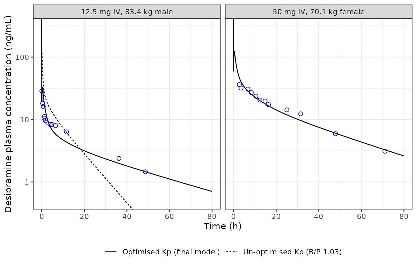
Replicates Figure 2a, 2c and 2d of Samant 2017: simulated venous plasma concentration (lines) against the deposited observed mean data (points). The dashed line is the un-optimised Kp set of Figure 2c.
The paper judged the adult model by the observed/predicted ratio of AUC over the observation window, accepting 0.8-1.25. The same ratio is computed below with PKNCA on both the deposited observations and the simulated profile, over each arm’s first-to-last observation time.
obs_win <- obs |>
  group_by(arm) |>
  summarise(start = min(time), end = max(time), .groups = "drop")

sim_auc <- bind_rows(sim_adult, sim_ap) |>
  mutate(treatment = paste(arm, scenario, sep = " | "))
obs_auc <- obs |>
  mutate(treatment = arm)

# The AUC window is each arm's first-to-last observation time; PKNCA's
# interval start/end bounds the integration, so the profiles are not trimmed.
auc_over_window <- function(conc_df) {
  conc_df <- dplyr::filter(conc_df, !is.na(Cc))
  dose_df <- conc_df |>
    distinct(treatment, arm) |>
    mutate(time = 0, dose = arm_dose[arm])
  conc_obj <- PKNCA::PKNCAconc(conc_df, Cc ~ time | treatment)
  dose_obj <- PKNCA::PKNCAdose(dose_df, dose ~ time | treatment)
  intervals <- conc_df |>
    distinct(treatment, arm) |>
    inner_join(obs_win, by = "arm") |>
    select(treatment, start, end) |>
    mutate(auclast = TRUE)
  res <- PKNCA::pk.nca(PKNCA::PKNCAdata(conc_obj, dose_obj, intervals = intervals))
  as.data.frame(res) |>
    filter(PPTESTCD == "auclast") |>
    select(treatment, auclast = PPORRES)
}

auc_obs <- auc_over_window(obs_auc) |> rename(arm = treatment, auc_obs = auclast)
auc_pred <- auc_over_window(sim_auc) |>
  tidyr::separate(treatment, into = c("arm", "scenario"), sep = " \\| ") |>
  rename(auc_pred = auclast)

auc_tab <- auc_pred |>
  inner_join(auc_obs, by = "arm") |>
  mutate(
    ratio = auc_obs / auc_pred,
    paper = case_when(
      scenario == "Optimised Kp (final model)" & grepl("^12.5", arm) ~ 0.97,
      scenario == "Optimised Kp (final model)" & grepl("^50", arm) ~ 0.87,
      TRUE ~ NA_real_
    )
  )
knitr::kable(
  auc_tab |>
    select(arm, scenario, auc_obs, auc_pred, ratio, paper) |>
    rename(
      "Arm" = arm, "Kp set" = scenario, "Observed AUC0-t (ng*h/mL)" = auc_obs,
      "Simulated AUC0-t (ng*h/mL)" = auc_pred, "Observed/simulated" = ratio,
      "Paper observed/predicted" = paper
    ),
  digits = 2
)| Arm | Kp set | Observed AUC0-t (ng*h/mL) | Simulated AUC0-t (ng*h/mL) | Observed/simulated | Paper observed/predicted |
|---|---|---|---|---|---|
| 12.5 mg IV, 83.4 kg male | Optimised Kp (final model) | 225.72 | 195.85 | 1.15 | 0.97 |
| 50 mg IV, 70.1 kg female | Optimised Kp (final model) | 815.22 | 769.75 | 1.06 | 0.87 |
| 12.5 mg IV, 83.4 kg male | Un-optimised Kp (B/P 1.03) | 225.72 | 253.61 | 0.89 | NA |
final_ratio <- auc_tab$ratio[auc_tab$scenario == "Optimised Kp (final model)"]
stopifnot(
  # Both adult arms meet the paper's own 0.8-1.25 acceptance criterion.
  all(final_ratio > 0.8 & final_ratio < 1.25)
)

# Terminal phase of the 12.5 mg arm: observed / simulated at the last two
# observations (36.28 and 48.69 h).
late <- obs |>
  filter(arm == "12.5 mg IV, 83.4 kg male", time > 30) |>
  left_join(
    bind_rows(sim_adult, sim_ap) |>
      filter(arm == "12.5 mg IV, 83.4 kg male") |>
      select(time, scenario, Cc_sim = Cc),
    by = "time"
  ) |>
  mutate(fold = Cc / Cc_sim)
late
#>                        arm  time   Cc                   scenario    Cc_sim
#> 1 12.5 mg IV, 83.4 kg male 36.28 2.39 Optimised Kp (final model) 1.9887818
#> 2 12.5 mg IV, 83.4 kg male 36.28 2.39 Un-optimised Kp (B/P 1.03) 0.6499343
#> 3 12.5 mg IV, 83.4 kg male 48.69 1.46 Optimised Kp (final model) 1.4602426
#> 4 12.5 mg IV, 83.4 kg male 48.69 1.46 Un-optimised Kp (B/P 1.03) 0.2125268
#>        fold
#> 1 1.2017407
#> 2 3.6772947
#> 3 0.9998339
#> 4 6.8697224
stopifnot(
  # The final Kp set carries the terminal phase.
  all(abs(log(late$fold[late$scenario == "Optimised Kp (final model)"])) < log(1.5)),
  # The un-optimised set (Vss about 4 L/kg) cannot: its terminal phase falls
  # several-fold below the observations.
  all(late$fold[late$scenario != "Optimised Kp (final model)"] > 3)
)
Both arms meet the paper’s acceptance band, but the ratios differ from the published ones (see Assumptions): the port distributes more slowly in the first hours than the published curves, with a brief lung-uptake hump in the first half hour and lower concentrations between about 4 and 12 h, while the terminal phase agrees.
The un-optimised Kp set reproduces the paper’s conclusion that the standard partitioning prediction cannot describe desipramine, but not the shape of Figure 2c. Its AUC over the observation window happens to fall inside the 0.8-1.25 band, while its terminal phase is far too steep (Vss of about 4 L/kg against a clearance held at 508 mL/h/kg). In Figure 2c the un-optimised curve instead lies above the late observations; there clearance comes from the platform’s CYP2D6 scaling, which this port does not reproduce, so the two scenarios are not expected to agree in shape.
Children: 12.5 mg IV from birth to adulthood
ped_ids <- c("M0", "M0.5", "M1", "M2.5", "M5", "M10", "M15", "M22")
ped_labels <- c(
  M0 = "0 wk", M0.5 = "0.5 years", M1 = "1 year", M2.5 = "2.5 years",
  M5 = "5 years", M10 = "10 years", M15 = "15 years", M22 = "22 years"
)
sim_ped <- bind_rows(lapply(ped_ids, sim_one, dose = 12.5, tend = 80)) |>
  mutate(age = factor(ped_labels[id], levels = ped_labels))
ggplot(sim_ped |> filter(time > 0), aes(time, Cc / 1000, colour = age)) +
  geom_line() +
  scale_y_log10() +
  labs(x = "Time (h)", y = "Concentration (mg/L)", colour = NULL) +
  theme_bw()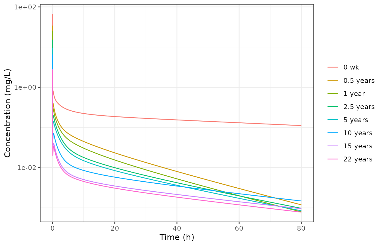
Replicates Figure 5 of Samant 2017: 12.5 mg IV desipramine in males of different ages (plasma, mg/L).
PKNCA: clearance and Vss for every deposited individual
Each deposited individual receives 12.5 mg IV and is followed for about seven or more terminal half-lives (720 h for newborns, whose half-life is near 90 h; 240 h otherwise). PKNCA recovers clearance and Vss (as CL x MRT) from the simulated profile. The clearance comparison is a numerical self-check, since clearance is anchored to the Supplementary Table; the Vss comparison is a check of the distribution model against the published value.
nca_ids <- subjects$id[!is.na(subjects$vss_kg) & subjects$id != "M34.5_ap"]
nca_tend <- ifelse(subjects$age[match(nca_ids, subjects$id)] < 0.1, 720, 240)
sim_all <- bind_rows(Map(sim_one, nca_ids, 12.5, nca_tend)) |>
  mutate(treatment = id, Cc_mgL = Cc / 1000)

conc_obj <- PKNCA::PKNCAconc(
  sim_all |> filter(!is.na(Cc_mgL)),
  Cc_mgL ~ time | treatment
)
dose_obj <- PKNCA::PKNCAdose(
  data.frame(treatment = nca_ids, time = 0, dose = 12.5),
  dose ~ time | treatment,
  route = "intravascular"
)
nca_res <- PKNCA::pk.nca(PKNCA::PKNCAdata(
  conc_obj, dose_obj,
  intervals = data.frame(
    start = 0, end = Inf, aucinf.obs = TRUE, cl.obs = TRUE, vss.obs = TRUE,
    half.life = TRUE
  )
))

wts <- setNames(subjects$wt, subjects$id)
sim_nca <- as.data.frame(nca_res) |>
  filter(PPTESTCD %in% c("cl.obs", "vss.obs")) |>
  mutate(PPORRES = ifelse(
    PPTESTCD == "cl.obs", PPORRES * 1000 / wts[treatment], PPORRES / wts[treatment]
  )) |>
  select(treatment, PPTESTCD, PPORRES)
ref_nca <- subjects |>
  filter(id %in% nca_ids) |>
  transmute(treatment = id, cl.obs = cl_kg, vss.obs = vss_kg)

cmp <- nlmixr2lib::ncaComparisonTable(
  sim_nca, ref_nca,
  by = "treatment",
  units = c(cl.obs = "mL/h/kg", vss.obs = "L/kg"),
  tolerance_pct = 20
)
# IV bolus: the clearance and volume are systemic, not apparent (/F).
cmp[["NCA parameter"]] <- sub("/F", "", cmp[["NCA parameter"]], fixed = TRUE)
knitr::kable(cmp, caption = attr(cmp, "footnote"))| NCA parameter | treatment | Reference | Simulated | % diff |
|---|---|---|---|---|
| CL (mL/h/kg) | M0 | 140 | 140 | -0.0% |
| CL (mL/h/kg) | F0 | 163 | 163 | -0.0% |
| CL (mL/h/kg) | M0.5 | 817 | 817 | -0.0% |
| CL (mL/h/kg) | F0.5 | 947 | 947 | -0.0% |
| CL (mL/h/kg) | M1 | 886 | 886 | -0.0% |
| CL (mL/h/kg) | F1 | 1030 | 1030 | -0.0% |
| CL (mL/h/kg) | M2.5 | 847 | 847 | -0.0% |
| CL (mL/h/kg) | F2.5 | 985 | 985 | -0.0% |
| CL (mL/h/kg) | M5 | 733 | 733 | -0.0% |
| CL (mL/h/kg) | F5 | 846 | 846 | -0.0% |
| CL (mL/h/kg) | M10 | 513 | 513 | -0.0% |
| CL (mL/h/kg) | F10 | 574 | 574 | -0.0% |
| CL (mL/h/kg) | M15 | 509 | 509 | -0.0% |
| CL (mL/h/kg) | F15 | 575 | 575 | -0.0% |
| CL (mL/h/kg) | M22 | 503 | 503 | -0.0% |
| CL (mL/h/kg) | F22 | 569 | 569 | -0.0% |
| CL (mL/h/kg) | M27 | 502 | 502 | -0.0% |
| CL (mL/h/kg) | F27 | 567 | 567 | -0.0% |
| CL (mL/h/kg) | M34.5 | 508 | 508 | -0.0% |
| CL (mL/h/kg) | F34.5 | 573 | 573 | -0.0% |
| Vss (L/kg) | M0 | 15.7 | 16.5 | +5.2% |
| Vss (L/kg) | F0 | 17.7 | 19.5 | +10.3% |
| Vss (L/kg) | M0.5 | 10.2 | 11.1 | +9.3% |
| Vss (L/kg) | F0.5 | 10.3 | 11.5 | +11.4% |
| Vss (L/kg) | M1 | 10.4 | 11.4 | +9.1% |
| Vss (L/kg) | F1 | 11 | 12.2 | +10.7% |
| Vss (L/kg) | M2.5 | 12.3 | 13.1 | +6.3% |
| Vss (L/kg) | F2.5 | 18.7 | 20.4 | +8.9% |
| Vss (L/kg) | M5 | 11.4 | 12 | +4.8% |
| Vss (L/kg) | F5 | 17 | 18.3 | +7.4% |
| Vss (L/kg) | M10 | 16.2 | 17 | +4.6% |
| Vss (L/kg) | F10 | 17.3 | 18.2 | +5.0% |
| Vss (L/kg) | M15 | 17.4 | 17.8 | +2.4% |
| Vss (L/kg) | F15 | 16.4 | 16.9 | +3.3% |
| Vss (L/kg) | M22 | 16.1 | 16.7 | +3.7% |
| Vss (L/kg) | F22 | 15.8 | 16.3 | +3.5% |
| Vss (L/kg) | M27 | 15.8 | 16.2 | +2.5% |
| Vss (L/kg) | F27 | 15.1 | 15.6 | +3.1% |
| Vss (L/kg) | M34.5 | 15.1 | 15.3 | +1.6% |
| Vss (L/kg) | F34.5 | 14.4 | 14.6 | +1.5% |
cl_pct <- sim_nca |>
  filter(PPTESTCD == "cl.obs") |>
  inner_join(ref_nca, by = "treatment") |>
  mutate(pct = 100 * (PPORRES - cl.obs) / cl.obs)
vss_pct <- sim_nca |>
  filter(PPTESTCD == "vss.obs") |>
  inner_join(ref_nca, by = "treatment") |>
  mutate(pct = 100 * (PPORRES - vss.obs) / vss.obs)
stopifnot(
  # Anchoring: the NCA clearance equals the Supplementary Table input. This
  # compares a solve against its own input, so the bound is tight.
  all(abs(cl_pct$pct) < 2),
  # Distribution: NCA Vss from the solved profile tracks the published Vss.
  abs(median(vss_pct$pct)) < 10,
  all(abs(vss_pct$pct) < 20)
)
The NCA Vss sits closer to the Supplementary Table than the algebraic
sum(Vt * Kp_t) above. For a model that eliminates drug in
the liver and kidney rather than from plasma, CL x MRT is smaller than
the sum of tissue volumes times Kp (Berezhkovskiy 2004, paper reference
33), and the closer agreement suggests the published Vss was derived the
same way from the simulated profiles.
Assumptions and deviations
- Hepatic clearance is anchored, not predicted. The paper derives hepatic intrinsic clearance from in vitro CYP2D6 kinetics (Vmax 68 pmol/min/mg, Km 6.1 uM; reference 21) through GastroPlus’s enzyme-expression scaling and built-in CYP2D6 ontogeny. Neither the scaling convention nor the ontogeny is documented in the paper or the deposited project, and the printed kinetics scaled with standard microsomal-protein factors fall roughly ten-fold short of the clearance the published profiles require. The maintainers anchored total plasma clearance to the Supplementary Table instead (within-paper sourcing: the value is the paper’s own simulated clearance for that age and sex). Consequently the model cannot be used to predict clearance in a new age group, phenotype or interaction scenario; Figure 4 is reproduced only by construction. Gut-wall CYP2D6 metabolism is omitted; the paper reports it as negligible (Discussion).
- The gut is a flow-through. The deposited physiology files carry the gut only as a reference to GastroPlus’s ACAT module, without a tissue volume or Kp, so blood perfusing the gut reaches the portal vein unchanged and the gut tissue contributes nothing to Vss. Including it would raise Vss further, so it does not account for the ~10% positive offset against the Supplementary Table.
- Oral dosing is not included (ACAT segments, absorption scale factors and the 0.55% enterocyte unbound fraction cannot be ported). The deposited compound database stores the enterocyte unbound fraction as 0.5%, against 0.55% in the text.
- Plasma unbound fraction is the Supplementary Table value (0.178 in adults; 0.178-0.239 in children), i.e. GastroPlus’s lipophilicity-adjusted fraction, not the unadjusted 0.19 of Table 1. It enters only renal clearance, which is about 3% of the total in adults.
-
Paediatric blood:plasma ratio is computed as
1 - HCT + HCT * E:Pwith the adult erythrocyte:plasma ratio held constant, which is how the paper describes the scaling (‘by accounting for age-dependent changes in hematocrit’); GastroPlus’s exact formula is not stated. Values range from 1.02 to 1.035. - Early distribution differs from the published curves. The paper reports observed/predicted AUC0-t of 0.97 (12.5 mg) and 0.87 (50 mg); this port gives the values in the table above. The port shows a brief rise in venous plasma concentration over the first half hour, as drug taken up by the lung on first pass is released, and distributes into muscle and the rest of the body (time constants of roughly 11 and 22 h) more slowly than the published curves suggest. No parameter was adjusted to close this gap; the deposited values are used as they are.
- The 50 mg IV individual is the deposited 70.1 kg, 30-year female (matching the observed-data file’s 70 kg); its clearance is interpolated between the 27- and 34.5-year female rows of the Supplementary Table.
- Population simulations are not reproduced. Figures 2b, 2e, 3b and 3e show GastroPlus Monte Carlo populations with 10-30% variability on system and drug parameters. The variability on the drug parameters is described only as ‘literature reported’, so the model is deterministic, with no between-subject or residual variability.
-
Tissue names. GastroPlus’s
ReproOrg,RedMarrowandYellowMarroware carried asreproductive_organs,red_marrowandyellow_marrow, andRestOfBodyasother. -
Untransformed
kp_*,vol_*andperf_*parameters. Every value is a fixed GastroPlus output, so the partition coefficients, volumes and flows are kept on their natural scale and in the deposited units (mL, mL/s); the naming check’s suggestion to log-transform thekp_*parameters is not applied. Each value then reads directly against the deposited files, and the per-individual table above can be passed torxSolve(params = ...)as is.