Lopinavir in Covid-19 (Alvarez 2021)
Source:vignettes/articles/Alvarez_2021_lopinavir.Rmd
Alvarez_2021_lopinavir.RmdModel and source
- Citation: Alvarez JC, Moine P, Davido B, Etting I, Annane D, Larabi IA, Simon N; Garches COVID-19 Collaborative Group. Population pharmacokinetics of lopinavir/ritonavir in Covid-19 patients. Eur J Clin Pharmacol. 2021;77(3):389-397. doi:10.1007/s00228-020-03020-w. The fixed ka, Imax and IC50 are taken from Dickinson L et al. Antimicrob Agents Chemother. 2011;55(6):2775-2782 (paper reference 10).
- Description: One-compartment first-order-absorption population PK model for oral lopinavir boosted by ritonavir (400/100 mg BID) in 13 hospitalised adults with Covid-19 (10 in intensive care). Apparent oral clearance CL/F is inhibited by the per-subject ritonavir trough concentration through a fixed Imax model, CL/F = CL0/F * (1 - Imax * C / (IC50 + C)), with ka, Imax and IC50 fixed to the Dickinson 2011 healthy-volunteer values. IIV on CL/F and V/F; residual error is proportional plus a fixed additive part (Alvarez 2021).
- Article: Eur J Clin Pharmacol. 2021;77:389-397
Alvarez et al. (2021) described lopinavir plasma concentrations in 13 hospitalised Covid-19 patients treated with lopinavir/ritonavir 400/100 mg twice daily. The final model is one-compartment with first-order absorption. The only retained covariate is the measured ritonavir trough concentration, which inhibits lopinavir apparent clearance through a maximum-inhibition model (Methods Equation 1):
CL/F = CL0/F x [1 - Imax x CresRTV / (IC50 + CresRTV)]
Because the data could not identify them, ka,
Imax and IC50 were fixed to the
healthy-volunteer estimates of Dickinson et al. 2011 (paper reference
10). In the packaged model the ritonavir trough is the covariate column
CONMED_RTV_CC (mg/L).
Population
Thirteen adults (4 female, 9 male; age 64 +/- 16 years, weight 85 +/-
15 kg, BMI 27.9 +/- 5.4 kg/m^2) admitted to Raymond Poincare Hospital,
Garches, France with confirmed Covid-19 contributed 70 lopinavir
concentrations (1 to 7 per patient; Table 1 and Results). Ten patients
were in intensive care, most intubated and ventilated, and received
crushed tablets by nasogastric tube. Ten had serum creatinine above the
laboratory normal range, and every patient had raised C-reactive
protein. Ritonavir troughs ranged from < 0.02 to 1.5 mg/L. Age,
weight, height, BMI, sex, creatinine, AST, ALT and CRP were tested and
not retained; they are recorded in the model’s
covariatesDataExcluded.
Source trace
| Model element | Value | Source |
|---|---|---|
| Structure: 1-compartment, first-order absorption, no lag | – | Results; Methods (ADVAN2) |
lka (fixed) |
log(0.572) 1/h | Table 2 ‘KA (fixed)’, from Dickinson 2011 |
lcl (CL0/F) |
log(4.88) L/h | Table 2 ‘CL0/F’ |
lvc (V/F) |
log(94.8) L | Table 2 ‘V/F’ |
ic50 (fixed) |
0.057 mg/L | Table 2 ‘IC50 (fixed)’, from Dickinson 2011 |
imax (fixed) |
0.929 | Table 2 ‘Imax (fixed)’, from Dickinson 2011 |
| CL/F inhibition equation | see above | Methods Equation 1; Table 2 footer |
etalcl |
2.881 (variance) | Table 2 IIV ‘CL’ |
etalvc |
0.801 (variance) | Table 2 IIV ‘V’ |
propSd |
0.186 | Table 2 RUV ‘Proportional’ |
addSd (fixed) |
0.071 mg/L | Table 2 RUV ‘Additive (fixed)’ |
| Residual form: proportional plus fixed additive | – | Results |
Scale of the variability parameters
Table 2 lists the random-effect estimates under the headings “omega” and “sigma” without saying whether they are variances or standard deviations.
IIV is a variance. Figure 4 and the Abstract report
that at steady state 40% of patients fall below the 16.7 mg/L target on
400 mg BID and 22% on 1200 mg BID. The model is linear, so tripling the
dose shifts log concentration by log(3) and the two percentages fix the
spread of log trough concentration independently of its median:
log(3) / (qnorm(0.40) - qnorm(0.22)). The chunk below
computes the model’s steady-state trough spread under both readings on a
deterministic quantile grid of the two etas.
cmin_ss <- function(cl, v, ka = 0.572, dose = 400, tau = 12) {
  k <- cl / v
  dose * ka / (v * (ka - k)) *
    (exp(-k * tau) / (1 - exp(-k * tau)) - exp(-ka * tau) / (1 - exp(-ka * tau)))
}
sd_paper <- log(3) / (qnorm(0.40) - qnorm(0.22))

grid_p <- (1:199) / 200
eta_grid <- expand.grid(a = qnorm(grid_p), b = qnorm(grid_p))
spread <- function(sd_cl, sd_v, rtv) {
  f <- 1 - 0.929 * rtv / (0.057 + rtv)
  cmin <- cmin_ss(4.88 * f * exp(sd_cl * eta_grid$a), 94.8 * exp(sd_v * eta_grid$b))
  c(sdlog = sd(log(cmin)), p400 = mean(cmin < 16.7), p1200 = mean(3 * cmin < 16.7))
}
iiv_check <- bind_rows(
  lapply(c(0.1, 0.2, 0.3), function(rtv) {
    rbind(
      data.frame(reading = "variance", rtv = rtv, t(spread(sqrt(2.881), sqrt(0.801), rtv))),
      data.frame(reading = "standard deviation", rtv = rtv, t(spread(2.881, 0.801, rtv)))
    )
  })
)
knitr::kable(
  iiv_check,
  digits = 3,
  caption = paste0(
    "Model steady-state trough spread under each reading. The paper's Figure 4 ",
    "percentages imply sdlog = ", signif(sd_paper, 3), " and a 40% -> 22% drop."
  )
)| reading | rtv | sdlog | p400 | p1200 |
|---|---|---|---|---|
| variance | 0.1 | 2.322 | 0.526 | 0.314 |
| standard deviation | 0.1 | 4.058 | 0.515 | 0.386 |
| variance | 0.2 | 2.168 | 0.435 | 0.238 |
| standard deviation | 0.2 | 3.920 | 0.461 | 0.335 |
| variance | 0.3 | 2.086 | 0.381 | 0.197 |
| standard deviation | 0.3 | 3.836 | 0.428 | 0.306 |
v_rows <- iiv_check[iiv_check$reading == "variance", ]
s_rows <- iiv_check[iiv_check$reading == "standard deviation", ]
stopifnot(
  all(abs(v_rows$sdlog - sd_paper) < 0.25),
  all(s_rows$sdlog > 1.5 * sd_paper)
)
The variance reading reproduces the implied spread (about 2.1) at every ritonavir level tried. The standard-deviation reading gives nearly twice that spread, and its 400 mg to 1200 mg drop is too small.
Residual error is a standard deviation. The additive term carries the unit mg/L in Table 2, which fits a standard deviation and not a variance. The supplementary DV-versus-IPRED plot shows most points within about 10% of identity and the largest near 30%. That fits a proportional SD of 18.6%. A 43% SD (the square root of 0.186) would put a sizeable share of points more than 40% from identity. This plot cannot rule that out as firmly as Figure 4 rules out the other IIV reading, because individual predictions absorb part of the residual error.
Typical apparent clearance versus ritonavir trough
mod <- readModelDb("Alvarez_2021_lopinavir")
rtv_levels <- c(0, 0.02, 0.057, 0.1, 0.2, 0.3, 0.5, 1.0, 1.5)
cl_tab <- data.frame(CONMED_RTV_CC = rtv_levels) |>
  mutate(
    cl_typ = 4.88 * (1 - 0.929 * CONMED_RTV_CC / (0.057 + CONMED_RTV_CC)),
    cavg_ss_400 = 400 / (12 * cl_typ)
  )
knitr::kable(
  cl_tab |>
    dplyr::rename(
      "Ritonavir trough (mg/L)" = CONMED_RTV_CC,
      "Typical CL/F (L/h)" = cl_typ,
      "Typical Cavg,ss at 400 mg BID (mg/L)" = cavg_ss_400
    ),
  digits = 2,
  caption = "Typical lopinavir CL/F across the observed ritonavir trough range."
)| Ritonavir trough (mg/L) | Typical CL/F (L/h) | Typical Cavg,ss at 400 mg BID (mg/L) |
|---|---|---|
| 0.00 | 4.88 | 6.83 |
| 0.02 | 3.70 | 9.00 |
| 0.06 | 2.61 | 12.76 |
| 0.10 | 1.99 | 16.73 |
| 0.20 | 1.35 | 24.66 |
| 0.30 | 1.07 | 31.14 |
| 0.50 | 0.81 | 41.13 |
| 1.00 | 0.59 | 56.41 |
| 1.50 | 0.51 | 65.05 |
stopifnot(
  abs(cl_tab$cl_typ[1] - 4.88) < 1e-9,
  abs(cl_tab$cl_typ[cl_tab$CONMED_RTV_CC == 0.057] - 4.88 * (1 - 0.929 / 2)) < 1e-9
)
The reported steady-state median of 20 to 30 mg/L (Figure 3) corresponds to a typical patient with a ritonavir trough of about 0.15 to 0.3 mg/L.
Steady-state identity check
A typical-value steady-state solve (ss = 1) must satisfy
AUCtau x CL/F = dose and match the closed-form trough.
mod_typ <- rxode2::zeroRe(mod)
#> ℹ parameter labels from comments will be replaced by 'label()'
rtv_chk <- c(0.1, 0.2, 0.3)
ev_ss <- bind_rows(lapply(seq_along(rtv_chk), function(i) {
  bind_rows(
    data.frame(id = i, time = 0, evid = 1, amt = 400, ii = 12, ss = 1, cmt = "depot"),
    data.frame(id = i, time = seq(0, 12, by = 0.05), evid = 0, amt = 0, ii = 0, ss = 0, cmt = "central")
  ) |>
    mutate(CONMED_RTV_CC = rtv_chk[i])
}))
sim_ss <- rxode2::rxSolve(mod_typ, ev_ss, returnType = "data.frame")
#> ℹ omega/sigma items treated as zero: 'etalcl', 'etalvc'
#> Warning: multi-subject simulation without without 'omega'
ss_tab <- sim_ss |>
  group_by(id) |>
  summarise(
    CONMED_RTV_CC = first(CONMED_RTV_CC),
    auc_tau = sum(diff(time) * (head(Cc, -1) + tail(Cc, -1)) / 2),
    cmin_sim = Cc[time == 12],
    cl = first(cl),
    .groups = "drop"
  ) |>
  mutate(
    dose_recovered = auc_tau * cl,
    cmin_closed = cmin_ss(cl, 94.8)
  )
knitr::kable(ss_tab, digits = 3)| id | CONMED_RTV_CC | auc_tau | cmin_sim | cl | dose_recovered | cmin_closed |
|---|---|---|---|---|---|---|
| 1 | 0.1 | 200.761 | 15.266 | 1.992 | 399.998 | 15.266 |
| 2 | 0.2 | 295.863 | 23.179 | 1.352 | 399.998 | 23.179 |
| 3 | 0.3 | 373.717 | 29.662 | 1.070 | 399.997 | 29.662 |
Virtual cohort
The paper does not report the distribution of ritonavir troughs used in its simulations. This vignette gives every virtual patient a ritonavir trough of 0.2 mg/L, which lies inside the observed range. With that value the typical steady-state concentrations fall in the paper’s reported 20-30 mg/L band. Each dose arm has 200 virtual patients. Doses are given every 12 h for 10 days, as in Figure 3.
rxode2::rxSetSeed(20210101)
n_per_arm <- 200
doses <- c(400, 800, 1200)
dose_times <- seq(0, 228, by = 12)
obs_times <- sort(unique(c(seq(0, 240, by = 2), seq(228, 240, by = 0.5))))

make_arm <- function(dose, arm_index) {
  ids <- (arm_index - 1) * n_per_arm + seq_len(n_per_arm)
  bind_rows(lapply(ids, function(i) {
    bind_rows(
      data.frame(id = i, time = dose_times, evid = 1, amt = dose, cmt = "depot"),
      data.frame(id = i, time = obs_times, evid = 0, amt = 0, cmt = "central")
    )
  })) |>
    mutate(CONMED_RTV_CC = 0.2, treatment = paste0(dose, " mg BID"))
}
events <- bind_rows(lapply(seq_along(doses), function(j) make_arm(doses[j], j))) |>
  arrange(id, time, desc(evid))

sim <- rxode2::rxSolve(mod, events, keep = "treatment", returnType = "data.frame")
#> ℹ parameter labels from comments will be replaced by 'label()'
Replicate Figure 3: 10 days of 400 mg BID
fig3 <- sim |>
  filter(treatment == "400 mg BID") |>
  group_by(time) |>
  summarise(
    med = median(Cc),
    lo = quantile(Cc, 0.05),
    hi = quantile(Cc, 0.95),
    .groups = "drop"
  )
ggplot(fig3, aes(time / 24, med)) +
  geom_ribbon(aes(ymin = lo, ymax = hi), alpha = 0.3) +
  geom_line() +
  geom_hline(yintercept = 16.7, linetype = "dashed") +
  scale_y_log10() +
  labs(x = "Time (days)", y = "Lopinavir concentration (mg/L)")
#> Warning in scale_y_log10(): log-10 transformation introduced infinite values.
#> log-10 transformation introduced infinite values.
#> log-10 transformation introduced infinite values.
#> log-10 transformation introduced infinite values.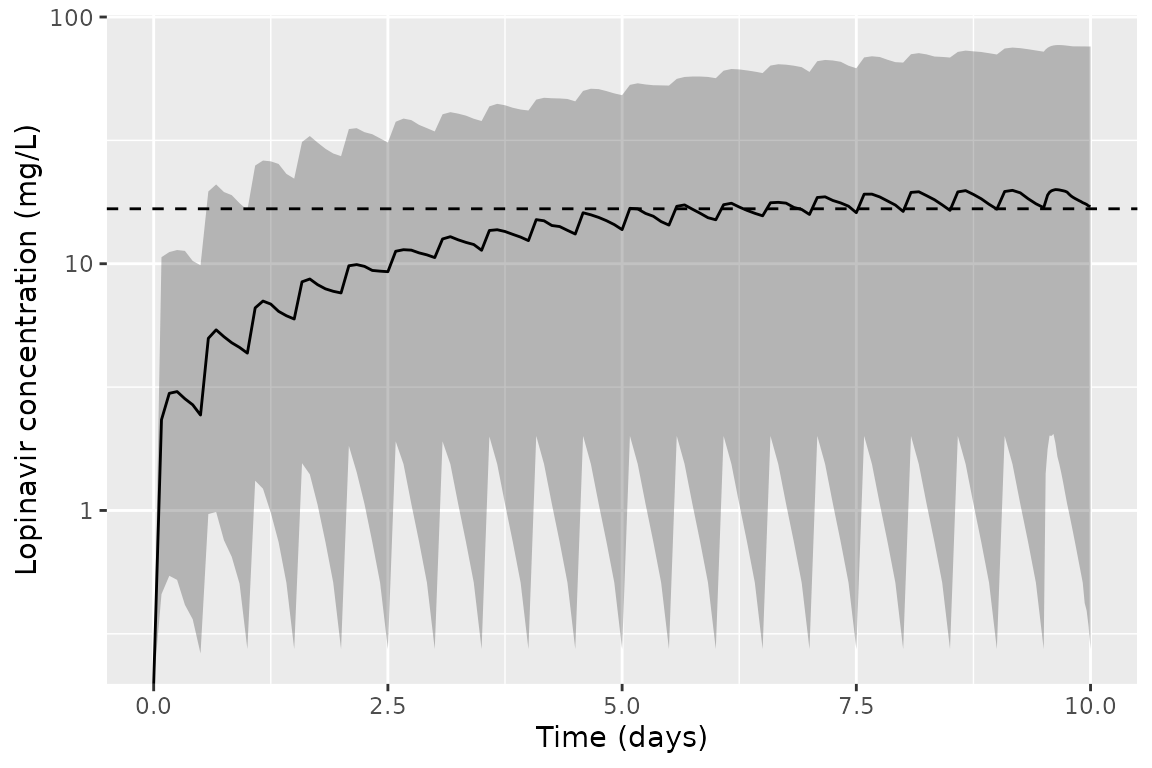
Replicates Figure 3 of Alvarez 2021: median (line) and 5th-95th percentile band of lopinavir concentration over 10 days of 400 mg BID. The dashed line is the 16.7 mg/L target.
The paper’s median settles between 20 and 30 mg/L, with a 90% prediction interval of roughly 1 to 100 mg/L.
last_day <- fig3 |> filter(time >= 228)
knitr::kable(last_day |> summarise(median_min = min(med), median_max = max(med), p5 = min(lo), p95 = max(hi)), digits = 1)| median_min | median_max | p5 | p95 |
|---|---|---|---|
| 16.9 | 20 | 0.3 | 77 |
# The cohort median of 200 patients moves by about +/-20% between random
# draws (log-scale IIV SD of 1.7 on CL/F), so the bound is wide: it catches a
# unit or clearance transcription error, not a 20% shift.
stopifnot(
  median(last_day$med) > 10,
  median(last_day$med) < 40
)
On day 10 the simulated median runs from about 17 to 20 mg/L over the dosing interval. That is a little below the paper’s band. The median of a cohort with this much variability in CL/F and V/F sits below the typical patient’s concentration, and the unknown ritonavir distribution adds further uncertainty.
Replicate Figure 4: fraction below the target by dose
troughs <- sim |>
  filter(time == 228) |>
  select(id, treatment, Cc)
ggplot(troughs, aes(Cc, colour = treatment)) +
  stat_ecdf() +
  geom_vline(xintercept = 16.7, linetype = "dashed") +
  scale_x_log10() +
  labs(x = "Lopinavir trough on day 10 (mg/L)", y = "Cumulative fraction of patients", colour = NULL)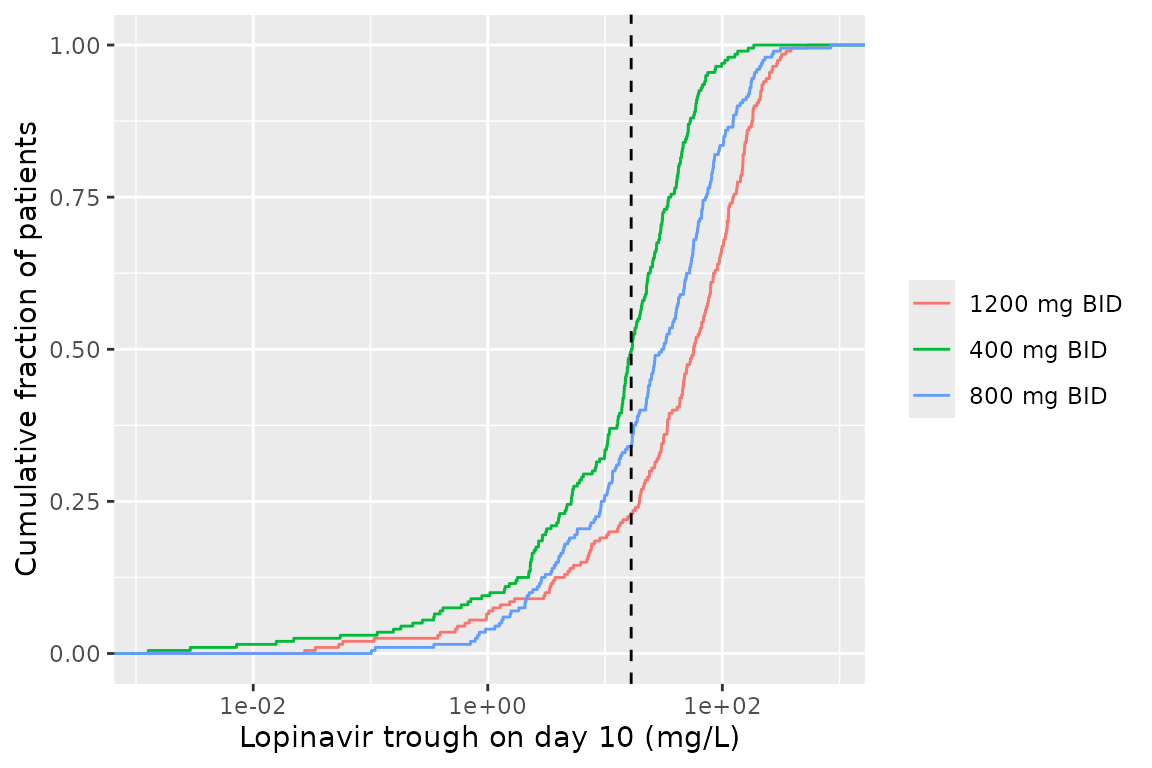
Replicates Figure 4 of Alvarez 2021: empirical cumulative distribution of the day-10 pre-dose (trough) concentration for each dose. The vertical dashed line is the 16.7 mg/L target.
below <- troughs |>
  group_by(treatment) |>
  summarise(pct_below = 100 * mean(Cc < 16.7), .groups = "drop")
knitr::kable(
  below |> dplyr::rename("Dose" = treatment, "Percent below 16.7 mg/L" = pct_below),
  digits = 1
)| Dose | Percent below 16.7 mg/L |
|---|---|
| 1200 mg BID | 23 |
| 400 mg BID | 50 |
| 800 mg BID | 34 |
The paper reports 40% below the target at 400 mg BID and 22% at 1200 mg BID. The simulated percentages depend on the assumed ritonavir trough. They also carry about 3.5 percentage points of sampling error with 200 patients per arm, and the day-10 troughs are not yet at steady state for the slowest-clearing patients. The fraction below the target at 400 mg is therefore higher than the paper’s. These percentages are shown for comparison and are not asserted. The deterministic spread check in “Scale of the variability parameters” is the test of the Figure 4 result.
PKNCA: steady-state interval on day 10
conc_df <- sim |>
  filter(time >= 228, !is.na(Cc)) |>
  select(id, time, Cc, treatment)
dose_df <- events |>
  filter(evid == 1, time == 228) |>
  select(id, time, amt, treatment)

conc_obj <- PKNCA::PKNCAconc(conc_df, Cc ~ time | treatment + id, concu = "mg/L", timeu = "h")
dose_obj <- PKNCA::PKNCAdose(dose_df, amt ~ time | treatment + id, doseu = "mg")
intervals <- data.frame(start = 228, end = 240, cmax = TRUE, cmin = TRUE, auclast = TRUE)
nca_res <- PKNCA::pk.nca(PKNCA::PKNCAdata(conc_obj, dose_obj, intervals = intervals))

nca_sum <- as.data.frame(nca_res$result) |>
  group_by(treatment, PPTESTCD) |>
  summarise(median = median(PPORRES), .groups = "drop") |>
  tidyr::pivot_wider(names_from = PPTESTCD, values_from = median)
knitr::kable(
  nca_sum |>
    dplyr::rename("Dose" = treatment, "Cmax (mg/L)" = cmax, "Cmin (mg/L)" = cmin, "AUC0-12 (mg*h/L)" = auclast),
  digits = 1,
  caption = "Median day-10 NCA metrics by dose (ritonavir trough 0.2 mg/L)."
)| Dose | AUC0-12 (mg*h/L) | Cmax (mg/L) | Cmin (mg/L) |
|---|---|---|---|
| 1200 mg BID | 738.9 | 65.0 | 56.9 |
| 400 mg BID | 223.4 | 20.0 | 16.9 |
| 800 mg BID | 418.5 | 36.8 | 31.0 |
Comparison against the published steady-state range
The paper gives only the median steady-state range: 20 mg/L at trough and 30 mg/L at peak (Abstract; Figure 3). That range comes from the paper’s own, unreported ritonavir distribution, so this comparison checks the order of magnitude and is not a precise test.
published <- data.frame(treatment = "400 mg BID", cmin = 20, cmax = 30)
cmp <- nlmixr2lib::ncaComparisonTable(
  simulated = nca_res,
  reference = published,
  by = "treatment",
  params = c("cmin", "cmax"),
  units = c(cmin = "mg/L", cmax = "mg/L"),
  tolerance_pct = 20
)
knitr::kable(cmp, caption = "Simulated 400 mg BID day-10 medians versus the published range. * marks rows differing by more than 20%.")| NCA parameter | treatment | Reference | Simulated | % diff |
|---|---|---|---|---|
| Cmax (mg/L) | 400 mg BID | 30 | 20 | -33.3%* |
| Cmin (mg/L) | 400 mg BID | 20 | 16.9 | -15.6% |
At a ritonavir trough of 0.2 mg/L the simulated median trough is about 16% below 20 mg/L. The simulated median peak, about 20 mg/L, is well below 30 mg/L. The model’s typical elimination half-life at this ritonavir level is about 48 h, so concentrations change little within a 12 h interval. The paper’s 20 to 30 mg/L range therefore most likely covers different patients or days, not the trough and peak of one dosing interval. The comparison is shown for orientation and is not asserted.
Assumptions and deviations
- IIV reported as variances, residual error as standard deviations. Table 2 does not state either scale. The IIV reading comes from the Figure 4 percentages (see “Scale of the variability parameters”). The residual reading comes from the mg/L unit on the additive term and the supplementary DV-versus-IPRED plot. IIV is taken as exponential (log-normal): the IIV on CL/F has a variance of 2.881, and a proportional (1 + eta) form would give negative clearances.
- Ritonavir trough units. The Methods text gives the unit as mg/mL. The Table 2 legend, the fixed IC50 and the reported range are all in mg/L, which is used here.
- Ritonavir trough distribution. Not reported. The simulations use a single value of 0.2 mg/L for every virtual patient. Users should supply measured or model-predicted ritonavir troughs.
- Time-fixed covariate. The model uses one ritonavir trough per patient, as the paper did. It does not simulate ritonavir concentrations over time.
-
Residual error form. “Proportional plus a fixed
additive part” is encoded as the nlmixr2 combined error
add(addSd) + prop(propSd). -
Dickinson 2011 parameters.
ka,ImaxandIC50are Dickinson 2011 healthy-volunteer values fixed by the authors. They were not re-estimated in Covid-19 patients.