Atezolizumab + cibisatamab colorectal cancer QSP (Ma 2020) • nlmixr2lib

# Build once and reuse: a 73-state model costs several seconds per build.
mod <- rxode2::rxode2(readModelDb("Ma_2020_atezolizumab_cibisatamab_qsp"))

Model and source

Citation: Ma H, Wang H, Sove RJ, Wang J, Giragossian C, Popel AS. Combination therapy with T cell engager and PD-L1 blockade enhances the antitumor potency of T cells as predicted by a QSP model. J Immunother Cancer. 2020;8(2):e001141. doi:10.1136/jitc-2020-001141.
Article: https://doi.org/10.1136/jitc-2020-001141

This is a deterministic quantitative systems pharmacology (QSP) model of microsatellite-stable (MSS) metastatic colorectal cancer treated with the anti-PD-L1 antibody atezolizumab, the CEA x CD3 bispecific T cell engager (TCE) cibisatamab, or both. It belongs to the Popel-laboratory immuno-oncology QSP family: the backbone is the non-small cell lung cancer model of Jafarnejad et al. (AAPS J 2019), the TCE module is that of Ma et al. (AAPS J 2020;22:85, the cibisatamab monotherapy paper), and this paper adds three updates described in its Supplementary Information:

PD-L2 with a weight delta (Supplementary Eqs 6-11): the number of PD-1/ligand complexes that drives T cell inhibition is PD1_PDL1 + delta * PD1_PDL2, in the Teff-cancer cell synapse and in the Teff-APC synapse. Atezolizumab blocks PD-L1 but not PD-L2.
PD-L1/PD-L2 on antigen-presenting cells limit T cell proliferation in the lymph node (Supplementary Eq 12): the proliferation of newly activated T cells is multiplied by 1 - H_PD1_APC, so atezolizumab acts during priming as well as in the tumour.
Teff killing rate combining the checkpoint and the TCE (Supplementary Eqs 13-14): basal Teff killing inhibited by H_PD1_C1, plus TCE-driven killing proportional to a Hill function of the CEA-cibisatamab-CD3 trimers.

The later Anbari 2023 platform (Anbari_2023_atezolizumab_cibisatamab_qsp) extends this model with myeloid-derived suppressor cells, T helper cells and cytokines; it is a separate model with its own parameter tables.

The authors built the model in SimBiology and published its SBML export as Supplementary file 2. The packaged model is a translation of that export (73 species, 105 reactions, 22 repeated-assignment rules, 12 initial assignments and one event), with the baseline values printed in Supplementary Tables S2 and S3 used wherever the export carries a different number (see Assumptions and deviations).

There are no etas and no residual-error model: the authors did not fit inter-individual variability. They generated 2000 virtual patients by Latin hypercube sampling of the Table S3 ranges. The model is packaged as the typical (Table S3 baseline) individual.

How the translation works

SimBiology converts units implicitly; rxode2 does not. Every value was converted to one consistent unit system – amounts in counts (the export defines 1 cell = 1 molecule = 1/Avogadro mol), volumes in litres, areas in dm^2, time in days – and each of the 105 rate laws, 22 rules and 12 initial assignments was checked by a dimensional-analysis pass that requires every rate to reduce to amount/time. The ODE states hold amounts, q_<compartment>_<species> (compartment and species names as in the export); the x_<compartment>_<species> variables are the SimBiology species values (concentrations for species stored as concentrations). Integrating amounts is what SimBiology does internally and handles the growing tumour volume without a dilution term. The reaction rates v1-v105 are numbered in the export’s reaction order, and each line of the model carries the reaction it encodes.

The two antibodies are held in nmol, so dose records are in nmol: atezolizumab into q_V_C_atezolizumab, cibisatamab into q_V_C_cibis (IV boluses). Every other state is a count.

Model outputs: tumour_diameter (cm, from the total tumour volume assuming a sphere), Cc_atezolizumab and Cc_cibisatamab (central concentrations, nmol/L), and the tumour-infiltrating cell densities teff_density and treg_density (cells per mL of tumour). The Hill terms H_PD1_C1, H_PD1_APC, H_CEA_C1_T1 and H_CEA_C1_T0 are also returned.

The pre-treatment phase

As in the paper, a simulation starts from a single cancer cell with no T cells anywhere and the tumour grows until it reaches the pre-treatment diameter; therapy then starts. The pre-treatment phase has no doses, so the untreated model is solved once to find the time at which the tumour reaches that diameter, and the first dose is scheduled at that time.

Population

The virtual population is described in the Results (“In silico VCT outcomes”). 2000 virtual patients were generated by Latin hypercube sampling of the parameters in Table S3 (tumour growth rate, initial tumour diameter 0.5-5 cm, tumour mutational burden, PD-1, PD-L1, PD-L2, CEA and CD3 expression, binding constants and cross-arm binding efficiencies). Patients were screened on tumour diameter, blood T cell density, activated T cell density in the tumour and the Teff/Treg ratio, leaving 1312 (atezolizumab 1200 mg Q3W), 1325 (cibisatamab 60 mg QW) and 1299 (combination) plausible patients. At day 400 the simulated objective response rates (ORR, RECIST 1.1) were 8.2, 5.2 and 11.2 percent, against 6 percent (cibisatamab, NCT02324257) and 12 percent (combination, NCT02650713) in the clinic (Table S4).

Source trace

Model element	Source
10 constant compartments (`vol_*`)	SBML export `listOfCompartments`
Model parameters (`ini()`; value and unit in each line’s comment)	SBML export `listOfParameters`; Supplementary Table S2 (atezolizumab-related variables) and Table S3 (sensitivity-analysis baselines) where printed
`K_PD1_PDLX` = 250 complexes	Table S2, `K_PD1_PDLX_CC` = `K_PD1_PDLX_APC` = 250 molecule
`delta_PDL2` = 1	Supplementary Eqs 10-11 (sampled on 0-1); the export’s Hill rules carry no weight
Checkpoint Hill terms `H_PD1_C1`, `H_PD1_APC`	Supplementary Eqs 6-11
T cell proliferation limited by `1 - H_PD1_APC` (`v9`, `v29`)	Supplementary Eq 12; SBML reactions 9 and 29
Teff killing of cancer cells (`v24`, `R_Tcell`)	Supplementary Eqs 13-14; SBML reaction 24
Atezolizumab binding to PD-L1 (`v78`, `v79`, `v84`, `v85`)	Supplementary Eqs 3-5; SBML reactions 78-79 and 84-85
Reaction rates `v1`-`v105`	SBML `kineticLaw` elements, in export order
Tumour volume `vol_V_T` and the other rules	SBML `listOfRules`
Initial amounts and synapse initial assignments	SBML `listOfSpecies` and `listOfInitialAssignments`
Cancer-cell elimination below 0.9 cells (`c1_alive`)	SBML `listOfEvents`
Regimens (atezolizumab 1200 mg Q3W, cibisatamab 60 mg QW, 400 days)	Results, “In silico VCT outcomes”
Atezolizumab plasma profile after 1200 mg	Supplementary Figure S1 (digitised by the maintainers)

Simulation set-up

# Dosing conversion for the vignette (not a model parameter). The paper gives
# doses in mg and no molar masses. Atezolizumab 145 kDa is the value used by the
# same group's atezolizumab QSP (Wang 2021, Supplementary Methods). No source
# gives the cibisatamab molar mass; 145 kDa is used as a carrier, see
# "Assumptions and deviations".
mw_kda <- c(atezolizumab = 145, cibisatamab = 145)
dose_nmol <- function(mg, drug) mg / (mw_kda[[drug]] * 1e3) * 1e6
atezo_nmol <- dose_nmol(1200, "atezolizumab")
cibis_nmol <- dose_nmol(60, "cibisatamab")

# method = "cvode" (SUNDIALS BDF). The stiff growth phase takes ~7 s per solve
# with lsoda and ~0.4 s with cvode; the final tumour diameters agree to about
# 1e-4 (relative).
SOLVE <- function(ev, params = NULL) {
  rxode2::rxSolve(mod, ev, params = params, method = "cvode", maxsteps = 1e6, returnType = "data.frame")
}

# Time at which the untreated tumour reaches diameter d0 (cm); NA if it never
# does (the immune system controls it, so the virtual patient has no tumour).
grow_to <- function(params = NULL, d0 = 3) {
  g <- SOLVE(rxode2::et(c(0, seq(1000, 9000, by = 10))), params = params)
  if (max(g$tumour_diameter) < d0) {
    return(NA_real_)
  }
  i <- which(g$tumour_diameter >= d0)[1]
  approx(g$tumour_diameter[(i - 1):i], g$time[(i - 1):i], d0)$y
}

# Treat from time ts for 400 days.
treat <- function(ts, atezo = FALSE, cibis = FALSE, params = NULL, obs = seq(0, 400, by = 4)) {
  ev <- rxode2::et(ts + obs)
  if (atezo) ev <- rxode2::et(ev, time = ts, amt = atezo_nmol, cmt = "q_V_C_atezolizumab", ii = 21, addl = 19)
  if (cibis) ev <- rxode2::et(ev, time = ts, amt = cibis_nmol, cmt = "q_V_C_cibis", ii = 7, addl = 57)
  s <- SOLVE(ev, params = params)
  s$day <- s$time - ts
  s
}

arm_def <- list(
  "Untreated" = c(atezo = FALSE, cibis = FALSE),
  "Atezolizumab" = c(atezo = TRUE, cibis = FALSE),
  "Cibisatamab" = c(atezo = FALSE, cibis = TRUE),
  "Combination" = c(atezo = TRUE, cibis = TRUE)
)
# Percentage change in tumour diameter at day 400 for each treated arm
pct400 <- function(params = NULL, d0 = 3, arms = names(arm_def)[-1]) {
  ts <- grow_to(params, d0)
  vapply(arms, function(a) {
    s <- treat(ts, arm_def[[a]][["atezo"]], arm_def[[a]][["cibis"]], params, obs = c(0, 400))
    100 * (s$tumour_diameter[s$day == 400] / d0 - 1)
  }, numeric(1))
}

Atezolizumab pharmacokinetics (Supplementary Figure S1)

Supplementary Figure S1 shows the atezolizumab plasma profile after a single 1200 mg dose, simulated and measured, with the measured points lying on the simulated curve. The points below were digitised by the maintainers. Both antibodies distribute in the same four compartments and are not consumed by their binding reactions (in the export the drug appears only in the rate law, never as a reactant), so their PK is linear and independent of the tumour; the doses are given at time zero.

fig_s1 <- data.frame(
  day = c(0, 3, 6, 9, 12, 15, 18, 21),
  conc = c(358, 209, 147, 120, 105, 96, 88, 81) # ug/mL, 1200 mg
)
pk_ev <- list(
  "Atezolizumab 1200 mg" = rxode2::et(seq(0, 21, by = 0.25)) |>
    rxode2::et(time = 0, amt = atezo_nmol, cmt = "q_V_C_atezolizumab"),
  "Cibisatamab 60 mg" = rxode2::et(seq(0, 21, by = 0.25)) |>
    rxode2::et(time = 0, amt = cibis_nmol, cmt = "q_V_C_cibis")
)
pk <- bind_rows(lapply(names(pk_ev), function(trt) {
  s <- SOLVE(pk_ev[[trt]])
  cc <- if (grepl("Atezo", trt)) s$Cc_atezolizumab else s$Cc_cibisatamab
  drug <- if (grepl("Atezo", trt)) "atezolizumab" else "cibisatamab"
  data.frame(treatment = trt, time = s$time, conc = cc * mw_kda[[drug]] * 1e3 / 1e6) # nmol/L -> ug/mL
}))
pk$id <- as.integer(factor(pk$treatment, levels = names(pk_ev)))

ggplot(pk, aes(time, conc, colour = treatment)) +
  geom_line(linewidth = 0.8) +
  geom_point(data = mutate(fig_s1, treatment = "Atezolizumab 1200 mg"), aes(day, conc)) +
  labs(x = "Time (days)", y = "Plasma concentration (ug/mL)", colour = NULL) +
  theme_bw() +
  theme(legend.position = "bottom")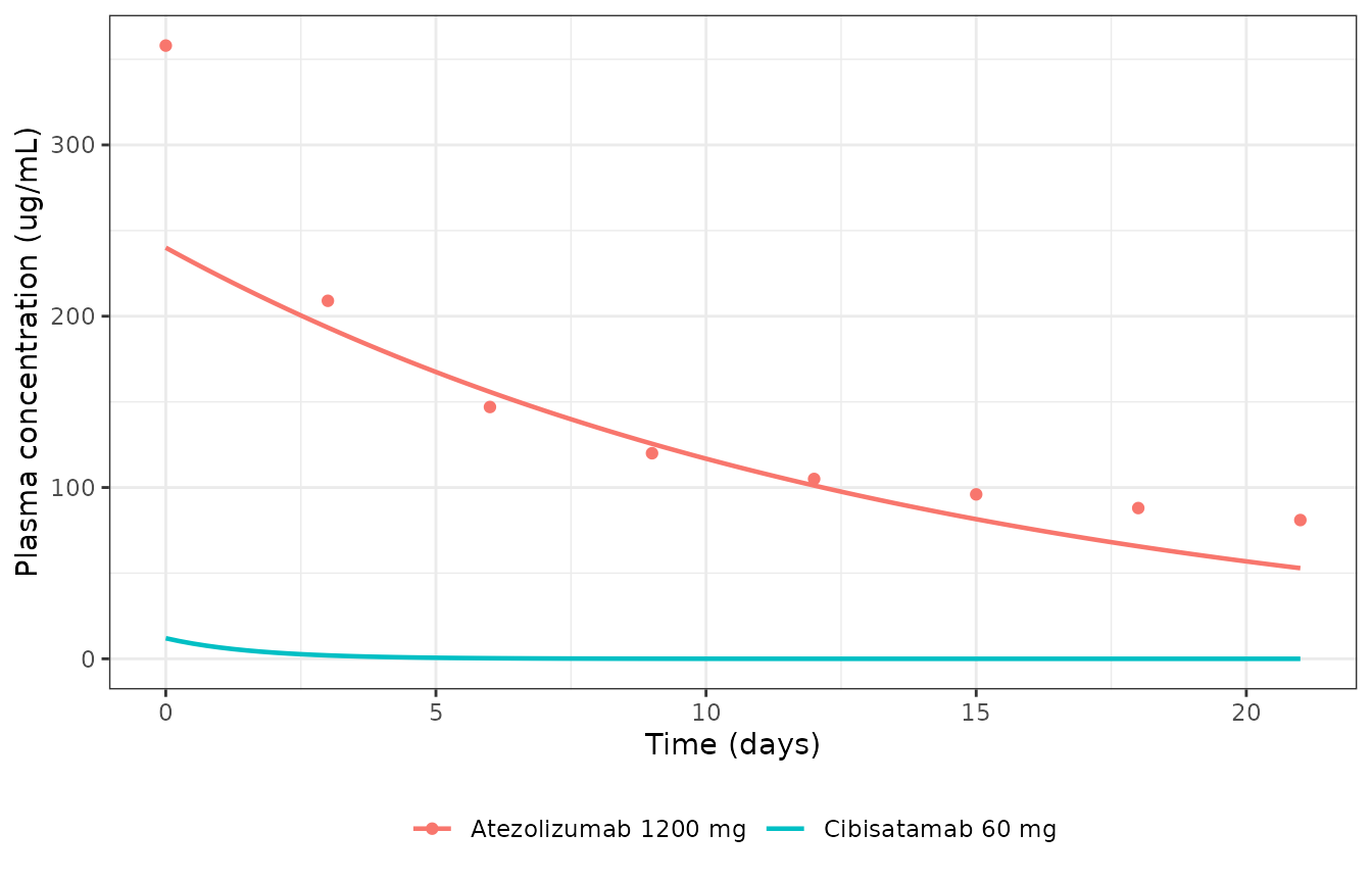

Atezolizumab plasma concentration after 1200 mg (line: packaged model) against Supplementary Figure S1 of Ma 2020 (points, digitised); cibisatamab after 60 mg for reference.

Non-compartmental analysis

conc_df <- pk |> select(id, treatment, time, conc)
dose_df <- conc_df |>
  distinct(id, treatment) |>
  mutate(time = 0, dose = c(1200, 60)[id])
o_conc <- PKNCA::PKNCAconc(conc_df, conc ~ time | treatment + id)
o_dose <- PKNCA::PKNCAdose(dose_df, dose ~ time | treatment + id)
intervals <- data.frame(start = 0, end = 21, cmax = TRUE, clast.obs = TRUE, auclast = TRUE)
nca <- PKNCA::pk.nca(PKNCA::PKNCAdata(o_conc, o_dose, intervals = intervals))

auc_fig <- sum(diff(fig_s1$day) * (head(fig_s1$conc, -1) + tail(fig_s1$conc, -1)) / 2)
reference <- data.frame(
  treatment = "Atezolizumab 1200 mg",
  cmax = fig_s1$conc[1],
  clast.obs = fig_s1$conc[8],
  auclast = auc_fig
)
tbl <- nlmixr2lib::ncaComparisonTable(
  nca, reference,
  by = "treatment",
  units = c(cmax = "ug/mL", clast.obs = "ug/mL", auclast = "day*ug/mL")
)
knitr::kable(tbl, caption = "Atezolizumab NCA over 0-21 days: Supplementary Figure S1 (Reference; digitised, AUC by the trapezoidal rule over its 3-day points) vs the packaged model (Simulated).")

Atezolizumab NCA over 0-21 days: Supplementary Figure S1 (Reference; digitised, AUC by the trapezoidal rule over its 3-day points) vs the packaged model (Simulated).
NCA parameter	treatment	Reference	Simulated	% diff
Cmax (ug/mL)	Atezolizumab 1200 mg	358	240	-33.0%*
Clast (ug/mL)	Atezolizumab 1200 mg	81	52.9	-34.7%*
AUClast (day*ug/mL)	Atezolizumab 1200 mg	2950	2600	-12.0%

nca_res <- as.data.frame(nca$result)
atz <- nca_res |> filter(treatment == "Atezolizumab 1200 mg")
cmax_sim <- atz$PPORRES[atz$PPTESTCD == "cmax"]
clast_sim <- atz$PPORRES[atz$PPTESTCD == "clast.obs"]
stopifnot(
  # The deposited model doses 1200 mg into the 5 L central volume: Cmax is
  # dose / V_C exactly, two-thirds of the 358 ug/mL drawn in Figure S1.
  abs(cmax_sim - 1200 / 5) < 0.5,
  # and the deposited clearance leaves about 53 ug/mL at day 21, not 81.
  abs(clast_sim / fig_s1$conc[8] - 0.65) < 0.05
)

Supplementary Figure S1 is not reproduced by the deposited atezolizumab PK. The figure starts at 358 ug/mL, which implies a central volume of about 3.3 L (the same 3.3 L follows from the 1, 3, 10 and 15 mg/kg curves at 70 kg), then shows a distribution phase and a slow terminal phase. The export’s central compartment is 5 L (vol_V_C), its central-peripheral flow q_P_atezolizumab is 7e-8 mL/s (6e-6 L/day, so there is effectively no peripheral distribution) and its elimination rate k_cl_atezolizumab is 0.003/h; the simulated profile therefore starts at 240 ug/mL and declines almost mono-exponentially with a 9.6-day half-life, to 53 against 81 ug/mL at day 21 (starred rows); the 0-21 day AUC is within 12 percent only because the simulated curve lies above the figure between days 4 and 11. The Supplementary text says the QSP PK was fitted to a two-compartment model of the clinical data, so the curves in Figure S1 are most likely that two-compartment fit rather than the deposited QSP. No value was changed: the PK parameters are those of the export, and Table S2 does not print them.

Reference virtual patient

The Table S3 baseline patient is grown from a single cancer cell to the Table S3 baseline pre-treatment diameter of 3 cm and treated for 400 days.

growth <- SOLVE(rxode2::et(c(0, seq(10, 6000, by = 10))))
t_star <- grow_to()
t_star
#> [1] 4497.749

ggplot(growth, aes(time / 365.25, tumour_diameter)) +
  geom_line() +
  geom_hline(yintercept = 3, linetype = "dashed") +
  scale_y_log10() +
  labs(x = "Time from the first cancer cell (years)", y = "Tumour diameter (cm)") +
  theme_bw()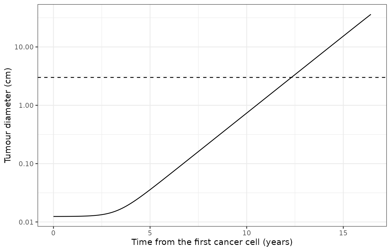

Untreated growth of the reference virtual patient from one cancer cell (tumour growth rate 0.005/day). The dashed line marks the 3 cm pre-treatment diameter.

arms <- bind_rows(lapply(names(arm_def), function(a) {
  s <- treat(t_star, arm_def[[a]][["atezo"]], arm_def[[a]][["cibis"]])
  s$arm <- a
  s
})) |>
  mutate(arm = factor(arm, levels = names(arm_def)), pct_change = 100 * (tumour_diameter / 3 - 1))
arm_sum <- arms |>
  group_by(arm) |>
  summarise(
    pct_end = pct_change[day == 400],
    teff_d56 = teff_density[day == 56],
    treg_d56 = treg_density[day == 56],
    h_pd1_c1_d56 = H_PD1_C1[day == 56],
    h_pd1_apc_d56 = H_PD1_APC[day == 56],
    h_tce_d56 = H_CEA_C1_T1[day == 56],
    .groups = "drop"
  )
arm_sum |>
  dplyr::rename(
    "Regimen" = arm, "Change in diameter at day 400 (%)" = pct_end,
    "Teff (cells/mL) at day 56" = teff_d56, "Treg (cells/mL) at day 56" = treg_d56,
    "H_PD1_C1 at day 56" = h_pd1_c1_d56, "H_PD1_APC at day 56" = h_pd1_apc_d56,
    "H_CEA_C1_T1 at day 56" = h_tce_d56
  ) |>
  knitr::kable(digits = 3, caption = "Reference virtual patient (Table S3 baselines, 3 cm) by regimen.")

Reference virtual patient (Table S3 baselines, 3 cm) by regimen.
Regimen	Change in diameter at day 400 (%)	Teff (cells/mL) at day 56	Treg (cells/mL) at day 56	H_PD1_C1 at day 56	H_PD1_APC at day 56	H_CEA_C1_T1 at day 56
Untreated	94.464	857.285	4403.614	0.999	1.000	0.00
Atezolizumab	94.377	1011.495	4155.292	0.751	0.997	0.00
Cibisatamab	94.356	856.637	4402.596	0.999	1.000	0.59
Combination	94.275	1011.320	4155.488	0.751	0.997	0.59

a <- setNames(split(arm_sum, arm_sum$arm), levels(arm_sum$arm))
stopifnot(
  # The baseline patient (tumour mutational burden 10) is progressive disease
  # under every regimen, the paper's most common outcome (80-87 percent PD).
  all(arm_sum$pct_end > 20),
  # Atezolizumab relieves PD-1 inhibition in the tumour and in the lymph node
  a[["Atezolizumab"]]$h_pd1_c1_d56 < a[["Untreated"]]$h_pd1_c1_d56 - 0.1,
  a[["Atezolizumab"]]$h_pd1_apc_d56 < a[["Untreated"]]$h_pd1_apc_d56,
  # and raises the intratumoral Teff density
  a[["Atezolizumab"]]$teff_d56 > 1.1 * a[["Untreated"]]$teff_d56,
  # Cibisatamab forms CEA-cibisatamab-CD3 trimers that engage the TCE Hill term
  a[["Cibisatamab"]]$h_tce_d56 > 0.3,
  a[["Untreated"]]$h_tce_d56 == 0
)

The baseline patient has a tumour mutational burden of 10 tumour-specific T cell clones, so few effector T cells are in the tumour when therapy starts (under 1000 per mL) and neither drug can control a 3 cm tumour. The mechanistic effects are nevertheless visible: atezolizumab lowers the PD-1 inhibition term in the tumour synapse (H_PD1_C1, from 0.999 to 0.75 – PD-L2, which atezolizumab does not block, keeps it high) and in the lymph-node synapse, and raises the Teff density; cibisatamab occupies the TCE Hill term.

ggplot(arms, aes(day, pct_change, colour = arm)) +
  geom_line(linewidth = 0.8) +
  geom_hline(yintercept = c(20, -30), linetype = "dashed") +
  labs(x = "Days from the start of therapy", y = "Change in tumour diameter (%)", colour = NULL) +
  theme_bw() +
  theme(legend.position = "bottom")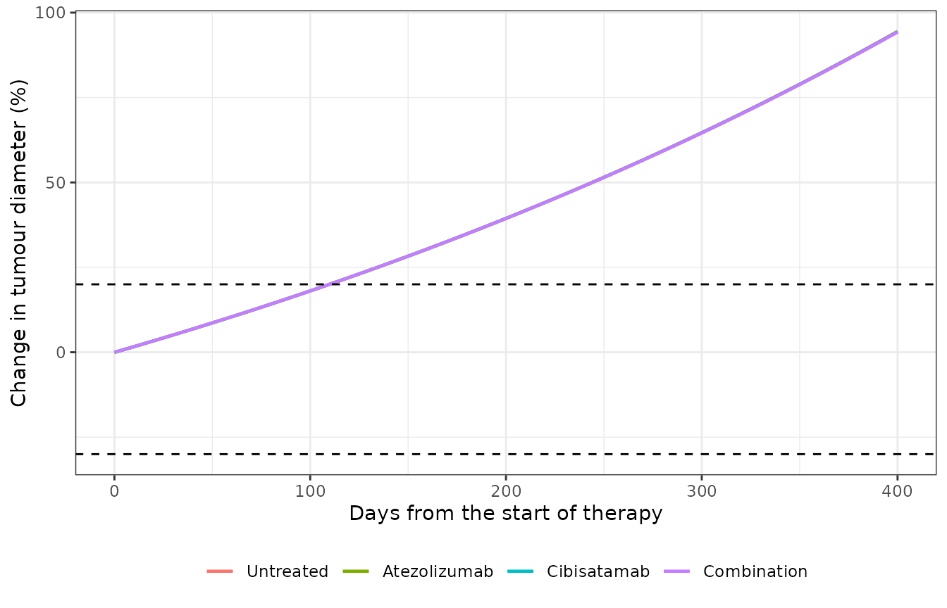

Reference virtual patient: change in tumour diameter under each regimen. Dashed lines: RECIST +20 percent (progression) and -30 percent (partial response).

Tumour mutational burden (Figures 2, 3A and 7B)

The paper identifies tumour mutational burden – in the model, the number of tumour-specific T cell clones n_T1_clones – as the strongest predictor of response under every regimen (partial rank correlation with tumour volume in Figure 2; ROC analysis in Figure 7A). In Figure 7B the ORR of patient subcohorts is close to 0 percent until the TMB exceeds about 76 and close to 100 percent above about 200, and the combination is the most active regimen. The reference patient is re-run across that range.

tmb_levels <- c(10, 80, 200, 500, 1000)
tmb <- bind_rows(lapply(tmb_levels, function(n) {
  p <- pct400(c(n_T1_clones = n))
  data.frame(tmb = n, arm = names(p), pct_end = unname(p))
})) |>
  mutate(arm = factor(arm, levels = names(arm_def)[-1]))
tmb |>
  pivot_wider(names_from = arm, values_from = pct_end) |>
  dplyr::rename("TMB (n_T1_clones)" = tmb) |>
  knitr::kable(digits = 1, caption = "Change in tumour diameter (%) at day 400 against tumour mutational burden, reference patient otherwise.")

Change in tumour diameter (%) at day 400 against tumour mutational burden, reference patient otherwise.
TMB (n_T1_clones)	Atezolizumab	Cibisatamab	Combination
10	94.4	94.4	94.3
80	88.8	89.1	80.7
200	67.7	70.0	33.0
500	6.8	12.1	-66.1
1000	-60.2	-50.6	-92.9

ggplot(tmb, aes(tmb, pct_end, colour = arm)) +
  geom_line() +
  geom_point() +
  geom_hline(yintercept = c(20, -30), linetype = "dashed") +
  scale_x_log10() +
  labs(x = "Tumour mutational burden (n_T1_clones)", y = "Change in diameter at day 400 (%)", colour = NULL) +
  theme_bw()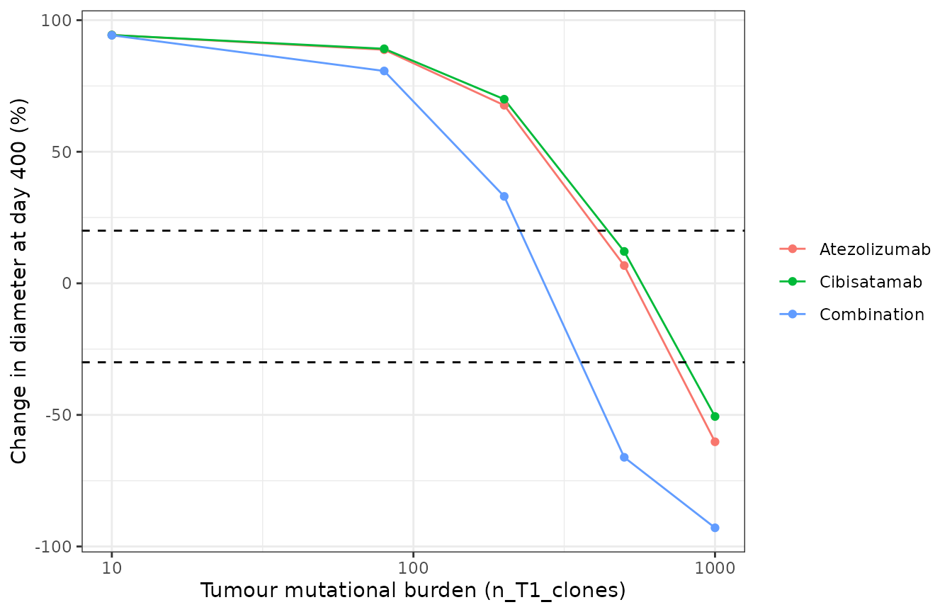

Change in tumour diameter at day 400 against tumour mutational burden for the three regimens (compare Figures 3A and 7B). Dashed lines: RECIST +20 and -30 percent.

w <- tmb |> pivot_wider(names_from = arm, values_from = pct_end)
stopifnot(
  # response improves monotonically with TMB under every regimen
  all(diff(w$Atezolizumab) < 0), all(diff(w$Cibisatamab) < 0), all(diff(w$Combination) < 0),
  # the combination is at least as active as either monotherapy at every TMB
  all(w$Combination <= pmin(w$Atezolizumab, w$Cibisatamab) + 0.01),
  # low TMB: progressive disease whatever the regimen
  all(unlist(w[w$tmb == 10, -1]) > 20),
  # TMB 500: the combination turns two progressing monotherapies into a
  # partial response (the paper's PD -> PR/CR group, Figure 5)
  w$Combination[w$tmb == 500] < -30,
  w$Atezolizumab[w$tmb == 500] > -30, w$Cibisatamab[w$tmb == 500] > -30,
  # TMB 1000: every regimen gives a RECIST response
  all(unlist(w[w$tmb == 1000, -1]) < -30)
)

CEA expression and tumour growth rate (Figure 2B)

Under the combination, CEA expression on cancer cells is negatively and the tumour growth rate positively correlated with tumour volume (Figure 2B). Both are checked one at a time at TMB 500, where the reference patient responds to the combination.

cea_levels <- c(1000, 20000, 300000) # Table S3 range and baseline
cea <- sapply(cea_levels, function(v) pct400(c(n_T1_clones = 500, C1_CEA_total = v), arms = "Combination"))
gr_levels <- c(0.005, 0.01)
gr <- sapply(gr_levels, function(v) pct400(c(n_T1_clones = 500, k_C1_growth = v), arms = "Combination"))
data.frame(
  scenario = c(paste("CEA", cea_levels, "per cell"), paste("growth rate", gr_levels, "1/day")),
  pct_end = c(cea, gr)
) |>
  dplyr::rename("Scenario (combination, TMB 500)" = scenario, "Change in diameter at day 400 (%)" = pct_end) |>
  knitr::kable(digits = 1)

Scenario (combination, TMB 500)	Change in diameter at day 400 (%)
CEA 1000 per cell	6.8
CEA 20000 per cell	-66.1
CEA 3e+05 per cell	-85.5
growth rate 0.005 1/day	-66.1
growth rate 0.01 1/day	-15.9

stopifnot(all(diff(cea) < 0), diff(gr) > 0)

PD-L2 weight delta (Supplementary Eqs 10-11)

The authors introduced delta because with PD-L2 tied to PD-L1 through a fixed ratio, responders appeared to carry more PD-L2; sampling delta on 0-1 changed the atezolizumab ORR from 8.2 to 9.3 percent. For a single patient the weight can matter much more, because PD-L2 is the part of the checkpoint signal that atezolizumab leaves untouched:

dl <- sapply(c(0, 1), function(d) pct400(c(n_T1_clones = 500, delta_PDL2 = d), arms = "Atezolizumab"))
data.frame(delta = c(0, 1), pct_end = dl) |>
  dplyr::rename("delta_PDL2" = delta, "Change in diameter at day 400 under atezolizumab, TMB 500 (%)" = pct_end) |>
  knitr::kable(digits = 1)

delta_PDL2	Change in diameter at day 400 under atezolizumab, TMB 500 (%)
0	-99.1
1	6.8

stopifnot(dl[1] < dl[2] - 50)

Parameter values of the SBML export (sensitivity scenario)

The SBML export carries different numbers from the printed baselines for eight parameters (listed under Assumptions and deviations). As a scenario only, the export’s values are restored here and the TMB comparison repeated. With them cibisatamab is almost inactive (its cross-arm efficiency lambda is 1 instead of 1000) and the Treg suppression rate is doubled, so even at TMB 1000 no regimen reaches a RECIST response – at odds with the paper’s response rates and with its Figure 7B. This is why the printed baselines are packaged.

deposit <- c(
  k_Treg = 2, C_PDL1_total = 4e5, r_PDL2C = 0.05, r_PDL2APC = 0.05,
  T1_CD3_total = 62000, T0_CD3_total = 62000,
  Chi_CEA_cibis = 0.333333330953227e8, # 0.3333 1/nm in 1/dm
  K_PD1_PDLX = 6 * 37.8 # PD1_50 = 6 molecule/um^2 over the 37.8 um^2 synapse
)
dep <- bind_rows(lapply(c(80, 500, 1000), function(n) {
  p <- pct400(c(deposit, n_T1_clones = n))
  data.frame(tmb = n, arm = names(p), pct_end = unname(p))
}))
dep |>
  pivot_wider(names_from = arm, values_from = pct_end) |>
  dplyr::rename("TMB (n_T1_clones)" = tmb) |>
  knitr::kable(digits = 1, caption = "Scenario with the SBML export's values (not the packaged model): change in tumour diameter (%) at day 400. TMB 80 is the export's own value.")

Scenario with the SBML export’s values (not the packaged model): change in tumour diameter (%) at day 400. TMB 80 is the export’s own value.
TMB (n_T1_clones)	Atezolizumab	Cibisatamab	Combination
80	93.3	94.4	93.2
500	72.1	93.3	70.7
1000	45.8	91.9	43.1

stopifnot(all(dep$pct_end > -30))

Mass conservation in the synapses

Receptor and ligand totals in each synapse are conserved by the binding reactions (the antibodies are not consumed). This is an exact identity of the ODE system, so it is checked tightly on the combination arm.

combo <- arms |> filter(arm == "Combination")
ini_val <- function(nm) mod$iniDf$est[mod$iniDf$name == nm]
syn_area <- 37.8 # um^2, Teff-cancer cell synapse
pdl1_0 <- ini_val("C_PDL1_total") / 897.270277791781 * syn_area # per cell / A_cell * synapse area
pdl1_tot <- with(combo, q_syn_T1_C1_PDL1 + q_syn_T1_C1_PD1_PDL1 + q_syn_T1_C1_PDL1_aPDL1 +
  2 * q_syn_T1_C1_PDL1_aPDL1_PDL1)
cea_0 <- ini_val("C1_CEA_total") / 1063.61760879936 * 75.6 # per cell / SA_cell * TCE synapse area
cea_tot <- with(combo, q_TCEsyn_T1_C1_CEA + q_TCEsyn_T1_C1_CEA_cibis + 2 * q_TCEsyn_T1_C1_CEA_cibis_CEA +
  q_TCEsyn_T1_C1_CEA_cibis_CD3 + 2 * q_TCEsyn_T1_C1_CEA_cibis_CEA_CD3)
cd3_0 <- ini_val("T1_CD3_total") / 151.310411930437 * 75.6
cd3_tot <- with(combo, q_TCEsyn_T1_C1_CD3 + q_TCEsyn_T1_C1_CD3_cibis + q_TCEsyn_T1_C1_CEA_cibis_CD3 +
  q_TCEsyn_T1_C1_CEA_cibis_CEA_CD3)
dev <- c(
  pdl1 = max(abs(pdl1_tot / pdl1_0 - 1)),
  cea = max(abs(cea_tot / cea_0 - 1)),
  cd3 = max(abs(cd3_tot / cd3_0 - 1))
)
dev
#>         pdl1          cea          cd3 
#> 2.581269e-13 6.340484e-13 3.054224e-12
stopifnot(all(dev < 1e-4))

Assumptions and deviations

Values that differ between the printed tables and the SBML export. The printed baselines are used, with the export’s value noted in each parameter’s comment:
- k_Treg = 1/day (export: 2/day, outside the Table S3 range 0.1-1);
- n_T1_clones (tumour mutational burden) = 10 (export: 80);
- C_PDL1_total = 160000 per cell (Tables S2 and S3; export: 400000, outside the Table S3 range 1-160000);
- r_PDL2C and r_PDL2APC = 0.065, the ratio of the Table S2 PD-L2 and PD-L1 totals (10400/160000 on cancer cells, 104000/1600000 on APCs; export: 0.05). Table S3 prints a baseline of 0.1, outside its own 0-0.07 range and the text’s 0.07 upper limit, so the Table S2 totals are taken;
- T1_CD3_total and T0_CD3_total = 61000 per cell (Table S3, and Ma 2020a Table S2; export: 62000);
- Chi_CEA_cibis = lambda / dT_syn with lambda = 1000 (Table S3, and Ma 2020a Tables S2 and S3; the export’s 0.3333/nm corresponds to lambda = 1);
- the PD-1 complex Hill constant is Table S2’s 250 complexes per synapse (K_PD1_PDLX); the export’s PD1_50 of 6 molecules/um^2 over the 37.8 um^2 synapse is 226.8.
The scenario above shows that the export’s values do not produce responders.
PD-L2 weight. The export has no delta; delta_PDL2 = 1 reproduces it, and the paper sampled delta on 0-1 only in a sensitivity rerun.
Atezolizumab PK. Not changed, although it does not reproduce Supplementary Figure S1 (see the PK section).
Exported formulas kept as they are. The atezolizumab concentration that binds PD-L1 in the Teff-APC (lymph node) synapse is the tumour concentration, divided by the lymph-node available fraction of cibisatamab (gamma_LN_cibis, numerically equal to gamma_LN_atezolizumab = 0.2); in the Teff-cancer cell synapse it is divided by the central available fraction gamma_C_atezolizumab rather than the tumour porosity of Supplementary Eq 3. TCE-driven killing through the Treg-cancer cell synapse multiplies the Teff count (k_C_BTreg term of v24). These are the export’s rate laws and are reproduced exactly.
Anti-PD-1 states. The export carries anti-PD-1 binding states and parameters from the backbone model with the anti-PD-1 concentration aPD1 set to 0; they are kept and stay at zero.
Unused export parameters (A_syn, SA_APC, T_syn, initial_tumour_diameter, kon_CD3_cibis2, kon_CEA_cibis2) are not carried; PD1_50 is replaced by K_PD1_PDLX.
Cancer-cell elimination event. SimBiology resets the cancer cell count to zero below 0.9 cells. rxode2 has no state-reset events, so proliferation is switched off below 0.9 cells (c1_alive) and the remaining fraction decays through the death terms.
Molar masses. No source gives them. Atezolizumab uses 145 kDa (the same group’s Wang 2021 atezolizumab QSP); cibisatamab uses 145 kDa as a carrier only. The cibisatamab dose in nmol therefore carries that assumption; Ma 2020a reports no ORR difference between 60 and 600 mg weekly, so the efficacy results are insensitive to it.
Virtual cohort. The paper’s ORRs come from 2000 Latin hypercube samples whose sampling distributions are not stated beyond the Table S3 ranges, so they are not re-simulated; the vignette checks the reported directions of effect on the baseline patient instead.
State names. States keep the SimBiology compartment.species naming (q_V_T_C1, q_syn_T1_C1_PD1, …) so each one can be traced to the export; they are not mapped onto the library’s PK compartment names.