Somatropin (Papathanasiou 2021)

Model and source

#> ℹ parameter labels from comments will be replaced by 'label()'

• Citation: Papathanasiou T, Agerso H, Damholt BB, Rasmussen MH, Kildemoes RJ. Population Pharmacokinetics and Pharmacodynamics of Once-Daily Growth Hormone Norditropin(R) in Children and Adults. Clin Pharmacokinet. 2021;60(9):1217-1226. doi:10.1007/s40262-021-01011-3

• Description: One-compartment population PK model with first-order absorption and zero-order endogenous GH production, linked to an indirect-response IGF-I model with an additive Emax stimulation of IGF-I production, for once-daily subcutaneous somatropin (Norditropin) in children and adults with growth hormone deficiency (Papathanasiou 2021)

• Article: https://doi.org/10.1007/s40262-021-01011-3 (open access, PMC8416863)

• Electronic supplementary material (ESM; Tables S1-S2 with the stepwise IIV and covariate search, Figures S1-S5): https://europepmc.org/article/PMC/PMC8416863

Somatropin (Norditropin, Novo Nordisk) is recombinant human growth hormone (GH) given as a once-daily subcutaneous injection for GH deficiency (GHD) in children and adults. Most of its therapeutic effect is mediated through serum insulin-like growth factor-I (IGF-I). Papathanasiou 2021 pooled the Norditropin comparator arms of three Novo Nordisk phase I trials and built a sequential PK/PD model: a GH PK model first, then an IGF-I indirect-response model with the PK parameters fixed at their PK-step estimates.

The paper’s point is that body weight explains the PK difference between children and adults: once weight is accounted for, no further child/adult PK difference remains. The IGF-I response keeps a separate adult and child Emax.

Population

Twenty-three subjects with GHD (Papathanasiou 2021 Table 1):

Trial	ClinicalTrials.gov	Population	n	Age, mean (range)	Weight, mean (range)	Norditropin regimen
1	NCT01973244	prepubertal children	8	8.2 y (6-11)	26.1 kg (17-39.8)	0.03 mg/kg once daily x 7 days
2	NCT00936403	prepubertal children	8	8.2 y (6-11)	29.7 kg (18-40.5)	0.035 mg/kg once daily x 7 days
3	NCT01706783	adults	7	58.0 y (23-68)	80.8 kg (59.1-102.2)	pre-trial dose (mean 0.0042 mg/kg) once daily x 4 weeks

Nineteen subjects were male and four female. Prior GH treatment was washed out for 7-14 days before the first dose. The analysis used 614 GH and 334 IGF-I concentrations. One adult was excluded for a suspected dosing error.

str(readModelDb("Papathanasiou_2021_somatropin")()$population)
#> List of 14
#>  $ species       : chr "human"
#>  $ n_subjects    : num 23
#>  $ n_studies     : num 3
#>  $ n_observations: chr "614 GH and 334 IGF-I concentrations"
#>  $ age_range     : chr "6-68 years (children 6-11 years; adults 23-68 years)"
#>  $ age_mean      : chr "23.4 years (children 8.2 years; adults 58.0 years)"
#>  $ weight_range  : chr "17-102.2 kg (children 17-40.5 kg; adults 59.1-102.2 kg)"
#>  $ weight_mean   : chr "44.0 kg (Trial 1 26.1 kg; Trial 2 29.7 kg; Trial 3 80.8 kg)"
#>  $ sex_female_pct: num 17.4
#>  $ race_ethnicity: chr "Not reported"
#>  $ disease_state : chr "Growth hormone deficiency (prepubertal children and adults), after a 7-14 day wash-out of prior GH treatment"
#>  $ dose_range    : chr "Once-daily subcutaneous Norditropin: 0.03 mg/kg for 7 days (Trial 1), 0.035 mg/kg for 7 days (Trial 2), and the"| __truncated__
#>  $ regions       : chr "Not reported in the article"
#>  $ notes         : chr "Pooled Norditropin comparator arms of three phase I trials: Trial 1 (NCT01973244, somapacitan, prepubertal chil"| __truncated__

Model structure

• GH PK (Figure 1; Table 2): one compartment, first-order absorption from the subcutaneous depot, linear elimination. A zero-order endogenous GH input K_Endo enters the central compartment. The model file sets it to c0 * CL/F, so that the pre-dose steady-state concentration equals the estimated baseline GH Base (c0). The central compartment starts at that steady state.
• Body weight (Methods section 2.6): P_i = P_typ * (BW / 70)^theta * exp(eta) on Ka (theta = -0.687), CL/F (0.982) and GH Base (-0.991). V/F has no weight effect. The absorption is flip-flop: ln(2) / 0.122 = 5.7 h is the apparent half-life.
• IGF-I (Figure 1; Table 3; Results section 3.3.1): indirect response with an additive Emax stimulation of the IGF-I production rate: d/dt(IGF1) = Kin + Emax * C / (EC50 + C) - Kout * IGF1, where C is the total (endogenous + exogenous) GH concentration.
• Emax by age group (Methods section 2.6): adults use Emax = 15.1 * (BW / 85)^0.46 (both fixed to the somapacitan estimates, because adult Emax was not identifiable at the single low adult dose). Children use Emax = 6.48 * (BW / 25)^1.94. One random effect is shared by both.
• Residual error: proportional throughout. GH has separate adult and child magnitudes, and IGF-I has a separate magnitude per trial, reflecting the different IGF-I assays.

Source trace

Element	Value in model	Source location
Structure (abs -> central, K_Endo, CL/F; IGF-I indirect response)	d/dt(depot), d/dt(central), d/dt(igf1)	Figure 1; Methods 2.4; Results 3.2.1, 3.3.1
Weight covariate form, 70 kg reference	(WT / 70)^e_wt_*	Methods 2.6, first displayed equation
Adult Emax form, 85 kg reference	(WT / 85)^e_wt_emax_adult	Methods 2.6, second displayed equation
Child Emax form, 25 kg reference	(WT / 25)^e_wt_emax_ped	Methods 2.6, third displayed equation
Age-group switch	(1 - CHILD) / CHILD	Methods 2.6, fourth displayed equation (adult = 1 - CHILD)
lka	log(0.122) 1/h	Table 2, Ka
lvc	log(28.2) L	Table 2, V/F
lcl	log(24.7) L/h	Table 2, CL/F
lc0	log(0.188) ng/mL	Table 2, GH Base
e_wt_cl, e_wt_ka, e_wt_c0	0.982, -0.687, -0.991	Table 2, theta BW rows
lkin	log(0.949) ng/mL/h	Table 3, Kin
lkout	log(0.0262) 1/h	Table 3, Kout
lec50	log(2.13) ng/mL	Table 3, EC50
lemax_adult, e_wt_emax_adult	fixed(log(15.1)), fixed(0.46)	Table 3, Emax adult and theta BW Emax adult (both fixed)
lemax_ped, e_wt_emax_ped	log(6.48), 1.94	Table 3, Emax child and theta BW Emax child
IIV Ka, V/F, CL/F, GH Base	CV 89.7%, 77.5%, 33.2%, 177%	Table 2, IIV CV column
IIV Kin, Kout, Emax	CV 117%, 17.4%, 33.1%	Table 3, IIV CV column
propSd_Cc_adult, propSd_Cc_ped	0.414, 0.561	Table 2, proportional error AGHD / GHD
propSd_IGF1_trial1/2/3	0.146, 0.087, 0.114	Table 3, proportional error Trial 1/2/3
IGF-I initial condition	(Kin + Emax * c0 / (EC50 + c0)) / Kout	Table 3 derived Kin,endo rows (checked below)

Structural checks

The paper’s derived endogenous IGF-I production rates

Table 3 prints two derived quantities: the IGF-I production rate at endogenous GH levels, Kin,endo = Kin + Emax * GHbase / (EC50 + GHbase). It is 1.97 ng/mL/h for an 85 kg adult and 2.22 ng/mL/h for a 25 kg child. Both depend jointly on Kin, EC50, both Emax values, GH Base, its weight exponent and the reference weights. The additive form, the 70/85/25 kg references and the use of total GH as the effect driver all have to be right to reproduce them. A proportional-effect reading, Kin * (1 + Emax * C / (EC50 + C)), gives 1.92 and 2.16 instead.

mod <- rxode2::rxode(readModelDb("Papathanasiou_2021_somatropin"))
#> ℹ parameter labels from comments will be replaced by 'label()'
th <- mod$theta

kin_endo <- function(wt, child) {
  c0 <- exp(th[["lc0"]]) * (wt / 70)^th[["e_wt_c0"]]
  emax <- if (child == 1) {
    exp(th[["lemax_ped"]]) * (wt / 25)^th[["e_wt_emax_ped"]]
  } else {
    exp(th[["lemax_adult"]]) * (wt / 85)^th[["e_wt_emax_adult"]]
  }
  exp(th[["lkin"]]) + emax * c0 / (exp(th[["lec50"]]) + c0)
}

kin_chk <- tibble::tibble(
  group = c("adult, 85 kg", "child, 25 kg"),
  model = c(kin_endo(85, 0), kin_endo(25, 1)),
  published = c(1.97, 2.22)
)
knitr::kable(kin_chk, digits = 3, caption = "Derived Kin,endo (ng/mL/h) vs Table 3.")

Derived Kin,endo (ng/mL/h) vs Table 3.

group	model	published
adult, 85 kg	1.974	1.97
child, 25 kg	2.224	2.22

# Deterministic arithmetic on the typical values: must agree to the two
# printed decimals.
stopifnot(all(abs(kin_chk$model - kin_chk$published) < 0.005))

Flip-flop half-life

Table 2’s footnote reports an apparent half-life of 5.6 h, ln(2) / 0.122. The absorption rate is slower than elimination, CL/F / V/F = 0.88 1/h at 70 kg.

ka70 <- exp(th[["lka"]])
kel70 <- exp(th[["lcl"]]) / exp(th[["lvc"]])
c(t_half_absorption = log(2) / ka70, t_half_elimination = log(2) / kel70)
#>  t_half_absorption t_half_elimination 
#>          5.6815343          0.7913664
stopifnot(abs(log(2) / ka70 - 5.68) < 0.01, kel70 > ka70)

Baseline hold without dosing

With no dose, GH must stay at its endogenous baseline and IGF-I at its endogenous steady state for any weight and age group.

mod_typ <- rxode2::zeroRe(mod)
#> Warning: No sigma parameters in the model

make_events <- function(ids, wt, child, study, dose_ug, ndose, obs_times) {
  do.call(rbind, lapply(seq_along(ids), function(i) {
    obs <- data.frame(
      id = ids[i], time = obs_times, amt = 0, evid = 0L,
      cmt = NA_character_, dvid = 1L
    )
    ev <- if (ndose > 0 && dose_ug[i] > 0) {
      rbind(
        data.frame(
          id = ids[i], time = (seq_len(ndose) - 1) * 24, amt = dose_ug[i],
          evid = 1L, cmt = "depot", dvid = NA_integer_
        ),
        obs
      )
    } else {
      obs
    }
    ev <- ev[order(ev$time, -ev$evid), ]
    ev$WT <- wt[i]
    ev$CHILD <- child[i]
    ev$STUDY_NCT00936403 <- study[i]
    ev
  }))
}

ev0 <- make_events(
  ids = 1:4, wt = c(17, 40, 60, 100), child = c(1, 1, 0, 0),
  study = c(0, 1, 0, 0), dose_ug = rep(0, 4), ndose = 0,
  obs_times = seq(0, 240, by = 24)
)
sim0 <- as.data.frame(rxode2::rxSolve(mod_typ, ev0, returnType = "data.frame"))
#> ℹ omega/sigma items treated as zero: 'etalka', 'etalvc', 'etalcl', 'etalc0', 'etalkin', 'etalkout', 'etalemax'
#> Warning: multi-subject simulation without without 'omega'
hold <- sim0 |>
  group_by(id) |>
  summarise(
    GH_range = diff(range(Cc)), IGF1_range = diff(range(IGF1)),
    GH = first(Cc), IGF1 = first(IGF1), .groups = "drop"
  )
knitr::kable(hold, digits = 4)

id	GH_range	IGF1_range	GH	IGF1
1	0	0	0.7643	67.1293
2	0	0	0.3273	118.2204
3	0	0	0.2190	82.0046
4	0	0	0.1320	72.4704

stopifnot(all(hold$GH_range < 1e-6), all(hold$IGF1_range < 1e-4))

The endogenous IGF-I baseline rises with weight in children (through the WT^1.94 pediatric Emax) and ranges from about 67 to 118 ng/mL over these four subjects. At the Table 1 mean weights (26.1 kg for Trial 1 children, 80.8 kg for adults), the typical baselines match the Day 0 geometric means read from Figure 2b, about 90 ng/mL for children and 80 ng/mL for adults:

ev_bl <- make_events(
  ids = 1:2, wt = c(26.1, 80.8), child = c(1, 0), study = c(0, 0),
  dose_ug = c(0, 0), ndose = 0, obs_times = 0
)
bl <- as.data.frame(rxode2::rxSolve(mod_typ, ev_bl, returnType = "data.frame"))
#> ℹ omega/sigma items treated as zero: 'etalka', 'etalvc', 'etalcl', 'etalc0', 'etalkin', 'etalkout', 'etalemax'
#> Warning: multi-subject simulation without without 'omega'
bl_chk <- tibble::tibble(
  group = c("child, 26.1 kg", "adult, 80.8 kg"),
  model = bl$IGF1, figure2b = c(90, 80)
) |>
  mutate(pct_diff = 100 * (model / figure2b - 1))
knitr::kable(bl_chk, digits = 1)

group	model	figure2b	pct_diff
child, 26.1 kg	87.3	90	-3.0
adult, 80.8 kg	76.3	80	-4.7

# Deterministic typical values against values read off a printed figure.
stopifnot(all(abs(bl_chk$pct_diff) < 15))

Virtual cohort

200 children (100 per pediatric trial) and 200 adults. Weights are drawn from normal distributions with the Table 1 means and SDs. The pediatric SD pools Trials 1 and 2. Draws outside the Table 1 range are rejected and redrawn, not clamped. Doses follow each trial’s per-kg regimen.

set.seed(20210417)
rxode2::rxSetSeed(20210417)
n_per_arm <- 200

draw_wt <- function(n, mean, sd, lo, hi) {
  out <- numeric(0)
  while (length(out) < n) {
    w <- rnorm(n, mean, sd)
    out <- c(out, w[w >= lo & w <= hi])
  }
  out[seq_len(n)]
}

wt_child <- draw_wt(n_per_arm, 28, 7.7, 17, 40.5)
wt_adult <- draw_wt(n_per_arm, 80.8, 18.2, 59.1, 102.2)
study2 <- rep(c(0, 1), length.out = n_per_arm)

obs_child <- sort(unique(c(seq(0, 96, by = 0.5), seq(96, 264, by = 1))))
obs_adult <- sort(unique(c(
  seq(0, 96, by = 0.5), seq(96, 624, by = 6), seq(624, 720, by = 0.5)
)))

ev_child <- make_events(
  ids = seq_len(n_per_arm), wt = wt_child, child = rep(1, n_per_arm),
  study = study2,
  dose_ug = ifelse(study2 == 1, 0.035, 0.03) * wt_child * 1000,
  ndose = 7, obs_times = obs_child
)
ev_adult <- make_events(
  ids = n_per_arm + seq_len(n_per_arm), wt = wt_adult,
  child = rep(0, n_per_arm), study = rep(0, n_per_arm),
  dose_ug = 0.0042 * wt_adult * 1000, ndose = 28, obs_times = obs_adult
)

sim <- bind_rows(
  as.data.frame(rxode2::rxSolve(mod, ev_child, returnType = "data.frame")) |>
    mutate(group = "Children with GHD"),
  as.data.frame(rxode2::rxSolve(mod, ev_adult, returnType = "data.frame")) |>
    mutate(group = "Adults with GHD")
)
sim |>
  distinct(id, group, WT) |>
  group_by(group) |>
  summarise(n = n(), WT_mean = mean(WT), WT_min = min(WT), WT_max = max(WT))
#> # A tibble: 2 × 5
#>   group                 n WT_mean WT_min WT_max
#>   <chr>             <int>   <dbl>  <dbl>  <dbl>
#> 1 Adults with GHD     200    80.0   59.2  102. 
#> 2 Children with GHD   200    29.2   17.2   40.1

Replication of Figure 2

Figure 2 shows geometric means with 95% CIs of the observed data and the geometric mean of the model predictions. The simulated bands below are 2.5th-97.5th percentiles of the individual predictions (random effects included, residual error excluded).

gm_band <- function(d, var) {
  d |>
    group_by(group, time) |>
    summarise(
      gm = exp(mean(log(.data[[var]]))),
      lo = quantile(.data[[var]], 0.025),
      hi = quantile(.data[[var]], 0.975),
      .groups = "drop"
    )
}

gh_sum <- gm_band(filter(sim, time <= 96), "Cc")
ggplot(gh_sum, aes(time / 24, gm, colour = group, fill = group)) +
  geom_ribbon(aes(ymin = lo, ymax = hi), alpha = 0.15, colour = NA) +
  geom_line(linewidth = 0.8) +
  scale_y_log10() +
  scale_colour_manual(values = c("Children with GHD" = "#1f3b73", "Adults with GHD" = "#56a0d3")) +
  scale_fill_manual(values = c("Children with GHD" = "#1f3b73", "Adults with GHD" = "#56a0d3")) +
  labs(x = "Time after first dose (days)", y = "GH (ng/mL)", colour = NULL, fill = NULL) +
  theme_bw() +
  theme(legend.position = "top")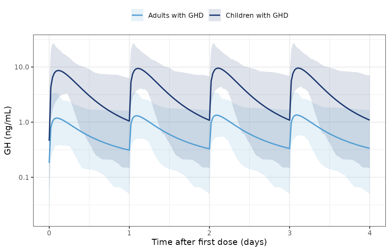

Replicates Figure 2a of Papathanasiou 2021: GH over the first 4 days of once-daily dosing.

igf_sum <- gm_band(filter(sim, time <= 264), "IGF1")
ggplot(igf_sum, aes(time / 24, gm, colour = group, fill = group)) +
  geom_ribbon(aes(ymin = lo, ymax = hi), alpha = 0.15, colour = NA) +
  geom_line(linewidth = 0.8) +
  scale_colour_manual(values = c("Children with GHD" = "#1f3b73", "Adults with GHD" = "#56a0d3")) +
  scale_fill_manual(values = c("Children with GHD" = "#1f3b73", "Adults with GHD" = "#56a0d3")) +
  coord_cartesian(ylim = c(0, 500)) +
  labs(x = "Time after first dose (days)", y = "IGF-I (ng/mL)", colour = NULL, fill = NULL) +
  theme_bw() +
  theme(legend.position = "top")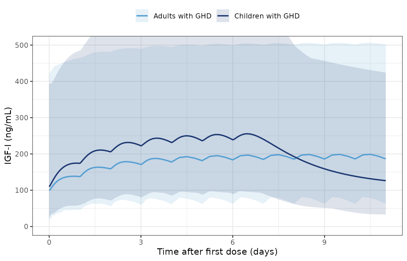

Replicates Figure 2b of Papathanasiou 2021: IGF-I over 7 (children) or 11 (adults) days.

Approximate values read from Figure 2 by the maintainers, against the simulated geometric means:

pick <- function(d, grp, var, t) {
  x <- d[d$group == grp & abs(d$time - t) < 1e-8, var]
  exp(mean(log(x)))
}
peak_gm <- function(grp) {
  gm_band(filter(sim, group == grp, time <= 24), "Cc") |>
    summarise(m = max(gm)) |>
    pull(m)
}
fig2 <- tibble::tibble(
  quantity = c(
    "GH peak, day 1 (ng/mL)", "GH trough at 24 h (ng/mL)",
    "IGF-I at 0 h (ng/mL)", "IGF-I on day 6 (ng/mL)"
  ),
  children_fig2 = c(10.5, 0.7, 90, 260),
  children_sim = c(
    peak_gm("Children with GHD"), pick(sim, "Children with GHD", "Cc", 24),
    pick(sim, "Children with GHD", "IGF1", 0), pick(sim, "Children with GHD", "IGF1", 144)
  ),
  adults_fig2 = c(1.1, 0.25, 80, 160),
  adults_sim = c(
    peak_gm("Adults with GHD"), pick(sim, "Adults with GHD", "Cc", 24),
    pick(sim, "Adults with GHD", "IGF1", 0), pick(sim, "Adults with GHD", "IGF1", 144)
  )
) |>
  mutate(
    children_pct_diff = 100 * (children_sim / children_fig2 - 1),
    adults_pct_diff = 100 * (adults_sim / adults_fig2 - 1)
  )
knitr::kable(fig2, digits = c(0, 2, 2, 2, 2, 0, 0))

quantity	children_fig2	children_sim	adults_fig2	adults_sim	children_pct_diff	adults_pct_diff
GH peak, day 1 (ng/mL)	10.5	8.64	1.10	1.18	-18	8
GH trough at 24 h (ng/mL)	0.7	1.05	0.25	0.31	49	24
IGF-I at 0 h (ng/mL)	90.0	109.76	80.00	99.45	22	24
IGF-I on day 6 (ng/mL)	260.0	238.96	160.00	183.69	-8	15

# Geometric means of a 200-subject cohort are centre statistics, but the
# day-1 GH peak and the IGF-I values still move by roughly +/-10% between
# cohort draws (rxode2 builds and thread counts draw different cohorts), and
# the reference values are read off a printed figure. The band is a factor of
# 1.5 either way. A dose or volume scaled by 1000, an Emax taken from the wrong
# age group or a proportional instead of additive effect moves these values
# by more than that. The 24 h GH trough is shown but not gated: it is a
# near-baseline value set largely by the 177% CV on GH Base.
gated <- c(fig2$children_sim[c(1, 3, 4)] / fig2$children_fig2[c(1, 3, 4)],
           fig2$adults_sim[c(1, 3, 4)] / fig2$adults_fig2[c(1, 3, 4)])
stopifnot(all(abs(log(gated)) < log(1.5)))

ev_tc <- make_events(
  ids = 1, wt = 26.1, child = 1, study = 0, dose_ug = 0.03 * 26.1 * 1000,
  ndose = 7, obs_times = 144
)
igf_typ_child <- as.data.frame(
  rxode2::rxSolve(mod_typ, ev_tc, returnType = "data.frame")
)$IGF1
#> ℹ omega/sigma items treated as zero: 'etalka', 'etalvc', 'etalcl', 'etalc0', 'etalkin', 'etalkout', 'etalemax'
igf_typ_child
#> [1] 176.6657

On day 6 the simulated geometric mean IGF-I is -8% from the Figure 2b value for children and 15% from it for adults. Both lie inside the observed 95% CIs of the figure. The typical-value prediction (all etas zero) for a 26.1 kg child on 0.03 mg/kg is lower, 177 ng/mL. With a 117% CV on Kin, the population average of the IGF-I profile is well above the profile of the typical subject. The same skew puts the simulated Day 0 geometric means above the typical baselines checked in the previous section.

Body weight and exposure (Figure 3)

With linear PK, the steady-state average concentration from the dose is Dose / (CL/F * 24), so the dose-normalised exposure falls with weight as WT^-0.982. Figure 3 plots this relationship: one weight curve covers both children and adults.

wt_grid <- seq(15, 105, by = 1)
cl_wt <- exp(th[["lcl"]]) * (wt_grid / 70)^th[["e_wt_cl"]]
fig3 <- tibble::tibble(WT = wt_grid, cavg_per_mg = 1000 / (cl_wt * 24))
ggplot(fig3, aes(WT, cavg_per_mg)) +
  geom_line(linewidth = 0.8) +
  labs(x = "Body weight (kg)", y = "Cavg,ss / dose (ng/mL per mg)") +
  theme_bw()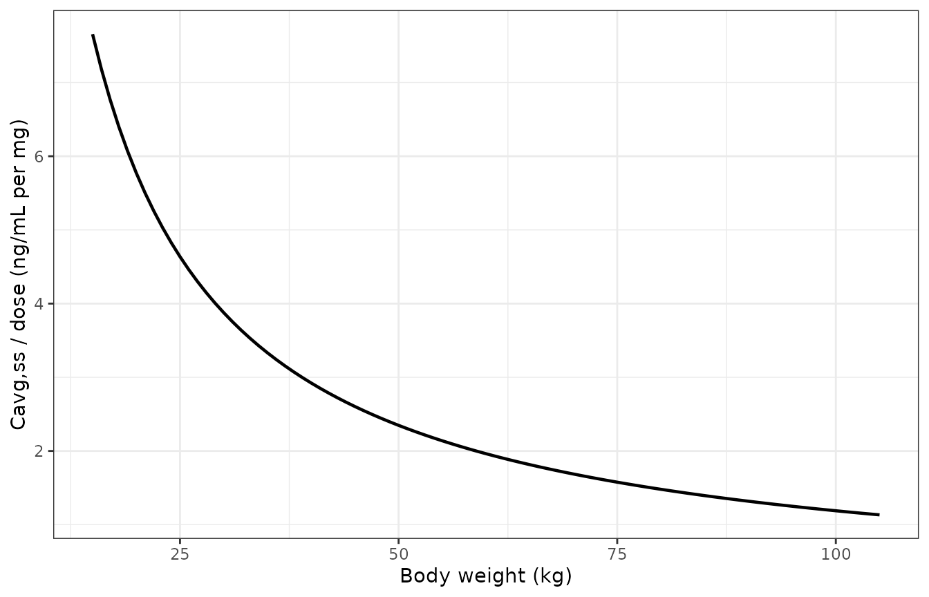

Replicates the population line of Figure 3 of Papathanasiou 2021: dose-normalised steady-state average GH (exogenous part) against body weight.

PKNCA validation

Non-compartmental analysis over the last dosing interval of each regimen: day 7 for children (144-168 h) and day 28 for adults (648-672 h).

sim_nca <- sim |>
  filter(!is.na(Cc)) |>
  select(id, time, Cc, group)

dose_df <- bind_rows(ev_child, ev_adult) |>
  filter(evid == 1) |>
  mutate(group = ifelse(CHILD == 1, "Children with GHD", "Adults with GHD")) |>
  select(id, time, amt, group)

conc_obj <- PKNCA::PKNCAconc(sim_nca, Cc ~ time | group + id)
dose_obj <- PKNCA::PKNCAdose(dose_df, amt ~ time | group + id)
intervals <- data.frame(
  group = c("Children with GHD", "Adults with GHD"),
  start = c(144, 648), end = c(168, 672),
  cmax = TRUE, tmax = TRUE, auclast = TRUE, cav = TRUE, cmin = TRUE
)
nca_res <- PKNCA::pk.nca(PKNCA::PKNCAdata(conc_obj, dose_obj, intervals = intervals))
nca_tab <- as.data.frame(nca_res)

nca_tab |>
  group_by(group, PPTESTCD) |>
  summarise(median = median(PPORRES), p5 = quantile(PPORRES, 0.05),
            p95 = quantile(PPORRES, 0.95), .groups = "drop") |>
  knitr::kable(digits = 2, caption = "Steady-state NCA of total GH (endogenous + exogenous).")

Steady-state NCA of total GH (endogenous + exogenous).

group	PPTESTCD	median	p5	p95
Adults with GHD	auclast	18.26	9.10	38.90
Adults with GHD	cav	0.76	0.38	1.62
Adults with GHD	cmax	1.44	0.66	3.33
Adults with GHD	cmin	0.37	0.08	1.27
Adults with GHD	tmax	2.00	1.00	5.00
Children with GHD	auclast	106.37	61.47	209.79
Children with GHD	cav	4.43	2.56	8.74
Children with GHD	cmax	10.04	4.89	23.62
Children with GHD	cmin	1.24	0.21	5.34
Children with GHD	tmax	3.00	1.00	6.05

Comparison against published values

The paper reports only an approximate time to maximum GH concentration: about 5.4 h in children and 2.1 h in adults (Results section 3.2.1). These were read from the observed profiles. It reports no Cmax or AUC.

published <- tibble::tibble(
  group = c("Children with GHD", "Adults with GHD"),
  tmax = c(5.4, 2.1)
)
cmp <- nlmixr2lib::ncaComparisonTable(
  simulated = nca_res,
  reference = published,
  by = "group",
  params = "tmax",
  units = c(tmax = "h"),
  tolerance_pct = 20
)
knitr::kable(cmp, caption = "Simulated vs. published Tmax. * differs from reference by >20%.")

Simulated vs. published Tmax. * differs from reference by >20%.

NCA parameter	group	Reference	Simulated	% diff
Tmax (h)	Children with GHD	5.4	3	-44.4%*
Tmax (h)	Adults with GHD	2.1	2	-4.8%

The adult Tmax agrees. The simulated pediatric Tmax is earlier than the reported 5.4 h. The printed value is an approximate figure read from sparsely sampled observed profiles: Trial 1 sampled at 1, 4 and 8 h, and Trial 2 at 0.25, 1, 2, 4, 6 and 8 h. A child whose true peak falls at 3 h is recorded at 4 h, and one whose peak falls after 4 h may be recorded at 6 or 8 h. So an observed Tmax is biased late compared with the continuous-time Tmax simulated here. The model gives children a faster absorption than adults (Ka scales as WT^-0.687) but a slower elimination (CL/F scales as WT^0.982 while V/F does not scale), and their Tmax is nevertheless later than adults’. That ordering matches the paper. No parameter is changed to match the printed value.

# Closed-form Tmax of the exogenous one-compartment first-order-absorption
# profile (the constant endogenous baseline does not move the peak).
tmax_cf <- function(wt) {
  ka <- exp(th[["lka"]]) * (wt / 70)^th[["e_wt_ka"]]
  kel <- exp(th[["lcl"]]) * (wt / 70)^th[["e_wt_cl"]] / exp(th[["lvc"]])
  log(ka / kel) / (ka - kel)
}
tmax_typ <- c(child_26kg = tmax_cf(26.1), adult_81kg = tmax_cf(80.8))
tmax_typ
#> child_26kg adult_81kg 
#>   3.522801   2.462152
stopifnot(tmax_typ[["child_26kg"]] > tmax_typ[["adult_81kg"]])

Exposure identity on a typical-value solve

For the typical subject, (AUCtau - c0 * tau) * CL/F must equal the dose at steady state, because the endogenous input contributes exactly c0 * tau to AUCtau. This deterministic check uses PKNCA on zeroRe() solves for four body weights.

wts <- c(20, 30, 70, 100)
ev_typ <- make_events(
  ids = seq_along(wts), wt = wts, child = c(1, 1, 0, 0), study = c(0, 1, 0, 0),
  dose_ug = c(0.03, 0.035, 0.0042, 0.0042) * wts * 1000, ndose = 14,
  obs_times = sort(unique(c(seq(0, 336, by = 0.25))))
)
sim_typ <- as.data.frame(rxode2::rxSolve(mod_typ, ev_typ, returnType = "data.frame"))
#> ℹ omega/sigma items treated as zero: 'etalka', 'etalvc', 'etalcl', 'etalc0', 'etalkin', 'etalkout', 'etalemax'
#> Warning: multi-subject simulation without without 'omega'
dose_typ <- ev_typ |> filter(evid == 1) |> select(id, time, amt)
nca_typ <- PKNCA::pk.nca(PKNCA::PKNCAdata(
  PKNCA::PKNCAconc(sim_typ, Cc ~ time | id),
  PKNCA::PKNCAdose(dose_typ, amt ~ time | id),
  intervals = data.frame(start = 312, end = 336, auclast = TRUE)
))
auc_typ <- as.data.frame(nca_typ) |>
  filter(PPTESTCD == "auclast") |>
  mutate(
    WT = wts[id],
    cl = exp(th[["lcl"]]) * (WT / 70)^th[["e_wt_cl"]],
    c0 = exp(th[["lc0"]]) * (WT / 70)^th[["e_wt_c0"]],
    dose = dose_typ$amt[match(id, dose_typ$id)],
    recovered_dose = (PPORRES - c0 * 24) * cl,
    pct_diff = 100 * (recovered_dose / dose - 1)
  )
knitr::kable(select(auc_typ, WT, dose, recovered_dose, pct_diff), digits = 3)

WT	dose	recovered_dose	pct_diff
20	600	599.731	-0.045
30	1050	1049.468	-0.051
70	294	293.826	-0.059
100	420	419.729	-0.064

# Same parameters on both sides; the only difference is trapezoidal error on a
# 0.25 h grid, so a tight bound is appropriate.
stopifnot(all(abs(auc_typ$pct_diff) < 1))

IGF-I at the Figure 4 matching doses

Figure 4 identifies 3 ug/kg/day for adults and 30 ug/kg/day for children as doses that give a matching average IGF-I SDS of about 1.1. The SDS transformation uses age- and sex-specific reference data (Bidlingmaier 2014) that are not part of this model, so only the IGF-I concentrations are shown. Children reach a higher IGF-I concentration at the matching SDS because their reference range is higher.

ev_f4 <- make_events(
  ids = 1:2, wt = c(25, 85), child = c(1, 0), study = c(0, 0),
  dose_ug = c(30 * 25, 3 * 85), ndose = 28,
  obs_times = seq(0, 28 * 24, by = 1)
)
sim_f4 <- as.data.frame(rxode2::rxSolve(mod_typ, ev_f4, returnType = "data.frame")) |>
  mutate(group = ifelse(id == 1, "Child, 25 kg, 30 ug/kg/day", "Adult, 85 kg, 3 ug/kg/day"))
#> ℹ omega/sigma items treated as zero: 'etalka', 'etalvc', 'etalcl', 'etalc0', 'etalkin', 'etalkout', 'etalemax'
#> Warning: multi-subject simulation without without 'omega'
ggplot(filter(sim_f4, time >= 24 * 21), aes((time - 24 * 21) / 24, IGF1, colour = group)) +
  geom_line(linewidth = 0.8) +
  labs(x = "Day of week 4", y = "IGF-I (ng/mL)", colour = NULL) +
  theme_bw() +
  theme(legend.position = "top")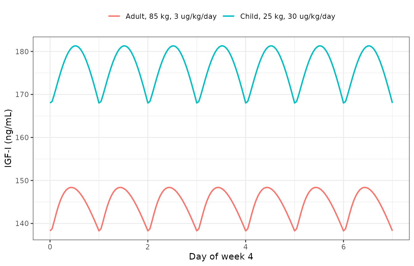

IGF-I (ng/mL) at steady state for a typical 25 kg child at 30 ug/kg/day and a typical 85 kg adult at 3 ug/kg/day (the Figure 4 dose levels).

wk4 <- sim_f4 |>
  filter(time >= 24 * 27) |>
  group_by(group) |>
  summarise(mean_IGF1 = mean(IGF1), .groups = "drop")
knitr::kable(wk4, digits = 1)

group	mean_IGF1
Adult, 85 kg, 3 ug/kg/day	144.3
Child, 25 kg, 30 ug/kg/day	175.8

# Deterministic: the child's steady-state IGF-I must exceed the adult's at the
# SDS-matched doses (Discussion: children need higher absolute IGF-I
# concentrations to reach the same SDS).
stopifnot(
  wk4$mean_IGF1[wk4$group == "Child, 25 kg, 30 ug/kg/day"] >
    wk4$mean_IGF1[wk4$group == "Adult, 85 kg, 3 ug/kg/day"]
)

Assumptions and deviations

• IIV correlations. The final PK model estimated Ka-CL/F and Ka-V/F correlations (ESM Table S1, dOFV -12.6), but their values are not reported in the article or the ESM. The model encodes independent random effects. This affects only the joint spread of simulated profiles, not typical-value predictions.
• CV to variance. Tables 2 and 3 report IIV as CV%. The variances use omega^2 = log(CV^2 + 1). The paper does not state which CV approximation it used. For the 177% CV on GH Base and 117% on Kin, the alternative omega = CV reading would give much larger variances (3.13 and 1.37 instead of 1.42 and 0.86).
• Initial conditions. The paper does not print the initial conditions. GH starts at its endogenous baseline and IGF-I at its endogenous steady state, (Kin + Emax * GHbase / (EC50 + GHbase)) / Kout. The Table 3 derived Kin,endo rows are exactly this production rate, and the resulting baselines match the Day 0 values in Figure 2b.
• Endogenous GH input. Figure 1 draws a zero-order input K_Endo into the central compartment, and Table 2 reports the baseline concentration it sustains (GH Base). The model writes the input as c0 * CL/F on the apparent (/F) amount scale. Predicted concentrations do not depend on this choice.
• Emax random effect. Table 3 prints the same 33.1% CV and 13.3% shrinkage on the adult and child Emax rows. This is read as one random effect shared by both typical values, matching the single eta_Emax in the Methods 2.6 equations.
• Subject count. The Results text says 15 children and 8 adults were eligible, then that one adult was excluded. Table 1 lists 8 + 8 children and 7 adults (23). The population metadata follows Table 1.
• Weight as a baseline covariate. The trials lasted at most 4 weeks, and the paper does not say whether weight varied with time. Weight is held constant per subject.
• Covariates. The paper’s adult indicator is encoded as CHILD = 1 - adult. The Trial 2 IGF-I residual error is selected by STUDY_NCT00936403. It matters only for children, because Trial 3, the only adult trial, is selected by CHILD = 0.
• Not reproduced. The IGF-I SDS transformation (Bidlingmaier 2014 reference data), and therefore the Figure 4 SDS axis, is outside the model.