Levamisole interspecies PK: allometric 2CM and minimal PBPK (Cheng 2026)

Model and source

Cheng, Jeong and Jusko (2026) assembled published levamisole (LVM) pharmacokinetic data from more than 40 papers spanning 18 species, digitized the concentration-time profiles, and fitted two joint interspecies models to the eight species that met their inclusion criteria (intravenous data available – except for humans – and warm-blooded). The paper contributes two structurally independent models, extracted here as two model files that share this vignette:

• Cheng_2026_levamisole_2cm – an allometric two-compartment model (Fig. 2, Table 2). Distribution is shared across species through simple allometric relations on body weight; elimination clearance is species-specific.
• Cheng_2026_levamisole_mpbpk – a minimal physiologically based model (Fig. 3, Table 3) with a blood compartment and two lumped tissue pools that split cardiac output and residual body volume. This is the model the authors preferred, on a lower AIC (598,377 versus 598,512).

Both fits are naive-pooled and deterministic (maximum likelihood in ADAPT 5 on one representative profile per species), so neither model carries between-subject variability.

• Article: https://doi.org/10.1007/s40005-025-00770-6
• Supplement (Tables S1-S10, Figures S1-S5): https://doi.org/10.1007/s40005-025-00770-6

mod_2cm <- readModelDb("Cheng_2026_levamisole_2cm")
mod_mpbpk <- readModelDb("Cheng_2026_levamisole_mpbpk")

rxode2::rxode2(mod_2cm)$reference
#> [1] "Cheng C, Jeong YS, Jusko WJ. Meta-analysis of levamisole absorption and disposition across diverse species using a minimal physiologically-based pharmacokinetic model. J Pharm Investig. 2026;56(2):171-183. doi:10.1007/s40005-025-00770-6."

Population

The analysis is a meta-analysis of the published literature rather than a study of a single cohort, so there is no subject-level demographic table to reproduce. The unit of analysis is the species: one representative single-dose profile was digitized per species so that every species contributes equal weight to the joint objective function, with the middle dose chosen for species studied over a dose range (rabbits and sheep). Inclusion required intravenous data (humans are the exception – only oral human data exist) and excluded cold-blooded species, whose much lower basal metabolic rate makes their clearance non-comparable.

pop <- rxode2::rxode2(mod_mpbpk)$meta$population
data.frame(
  Field = c("Species", "Studies", "Weight range", "Dose range"),
  Value = c(pop$species, as.character(pop$n_studies), pop$weight_range, pop$dose_range)
) |>
  knitr::kable()

Field	Value
Species	duck + rabbit + chicken + goat + dog + sheep + pig + human (joint interspecies fit; human is the model’s reference species)
Studies	8
Weight range	2.5-70 kg (one typical body weight per species; Table 1)
Dose range	Intravenous single doses of 5-40 mg/kg in the animal species and single oral doses of 50-150 mg in humans (Supplemental Tables S2, S3 and S4).

The eight modelled species, their body weights, and the intravenous profile each contributed are below. Body weights are the typical values the joint fit used (Table 1 and Supplemental Table S1C); doses and source studies are from Supplemental Table S2 (rows footnoted “Data used for 2CM and mPBPK modeling”).

species_tbl <- tibble::tribble(
  ~species,   ~wt,   ~iv_mgkg, ~source,
  "Duck",       2.5,  30,   "Tabari 2022",
  "Rabbit",     3.0,  16.0, "Villanueva 2003 (middle of 12.5/16/20)",
  "Chicken",    4.5,  40,   "El-Kholy 2006",
  "Goat",      18.0,   5,   "Nielsen & Rasmussen 1983",
  "Dog",       20.7,  10,   "Watson 1988",
  "Sheep",     26.0,   7.5, "Fernandez 1997 (middle of 5/7.5/10)",
  "Pig",       39.2,   5,   "Galtier 1983",
  "Human",     70.0,  NA,   "no IV data; oral only (Table S4)"
) |>
  mutate(iv_dose_mg = iv_mgkg * wt)

sp_levels <- species_tbl$species

species_tbl |>
  rename(
    "Species" = species, "Body weight (kg)" = wt, "IV dose (mg/kg)" = iv_mgkg,
    "IV dose (mg)" = iv_dose_mg, "Source study" = source
  ) |>
  knitr::kable(digits = 1)

Species	Body weight (kg)	IV dose (mg/kg)	Source study	IV dose (mg)
Duck	2.5	30.0	Tabari 2022	75
Rabbit	3.0	16.0	Villanueva 2003 (middle of 12.5/16/20)	48
Chicken	4.5	40.0	El-Kholy 2006	180
Goat	18.0	5.0	Nielsen & Rasmussen 1983	90
Dog	20.7	10.0	Watson 1988	207
Sheep	26.0	7.5	Fernandez 1997 (middle of 5/7.5/10)	195
Pig	39.2	5.0	Galtier 1983	196
Human	70.0	NA	no IV data; oral only (Table S4)	NA

Source trace

Every value in both ini() blocks, and every non-trivial model() equation, with the location in Cheng 2026 it came from.

tibble::tribble(
  ~Model, ~Quantity, ~Value, ~Source,
  "2CM",   "a1, b1 (central volume Vp allometry)",     "0.339 L, 1.309",      "Table 2",
  "2CM",   "a2, b2 (peripheral volume Vt allometry)",  "0.937 L, 0.885",      "Table 2",
  "2CM",   "a3, b3 (distributional clearance CLd)",    "0.352 L/h, 0.920",    "Table 2",
  "2CM",   "ka (human oral)",                          "1.702 /h",            "Table 2",
  "2CM",   "F (human oral, fixed)",                    "0.66",                "Table 2; Absorption kinetics",
  "2CM",   "CL by species",                            "0.20-1.09 L/h/kg",    "Table 1, 'Joint 2CM' column",
  "2CM",   "Disposition ODEs",                         "Vp dCp/dt, Vt dCt/dt","Eqs. (3), (4)",
  "mPBPK", "Kp (shared)",                              "1.41",                "Table 3",
  "mPBPK", "Kp,pig / Kp,chicken",                      "5.62 / 3.38",         "Table 3",
  "mPBPK", "ft (tissue-1 volume fraction)",            "0.497",               "Table 3",
  "mPBPK", "fd1 / fd2",                                "0.038 / 0.962",       "Table 3",
  "mPBPK", "fd,total (fixed)",                         "1.0",                 "Table 3; Eq. (11)",
  "mPBPK", "Rb (assumed)",                             "1",                   "Methods, basic PK parameters",
  "mPBPK", "Cardiac output",                           "14.1 * BW^0.75 L/h",  "Eq. (8); Table S1C",
  "mPBPK", "Blood volume by species",                  "50.9-100 mL/kg",      "Supplemental Table S1A",
  "mPBPK", "Tissue volumes V1, V2",                    "(BW - Vb) * ft, * (1-ft)", "Eqs. (9), (10)",
  "mPBPK", "CL by species",                            "0.216-2.59 L/h/kg",   "Table 1, 'Joint mPBPK' column",
  "mPBPK", "ka (human oral)",                          "1.156 /h",            "Supplemental Table S7 footnote b (see Errata)",
  "mPBPK", "F (human oral, fixed)",                    "0.66",                "Absorption kinetics",
  "mPBPK", "Disposition ODEs",                         "Vb Rb dCp/dt, V1 dC1/dt, V2 dC2/dt", "Eqs. (5), (6), (7)",
  "both",  "Absorption compartment",                   "dAa/dt = -ka * Aa",   "Eq. (12)",
  "both",  "Residual error form",                      "Var = (sigma1 + sigma2*Y)^2", "Methods, Model fitting (magnitudes unpublished; see Errata)"
) |>
  knitr::kable()

Model	Quantity	Value	Source
2CM	a1, b1 (central volume Vp allometry)	0.339 L, 1.309	Table 2
2CM	a2, b2 (peripheral volume Vt allometry)	0.937 L, 0.885	Table 2
2CM	a3, b3 (distributional clearance CLd)	0.352 L/h, 0.920	Table 2
2CM	ka (human oral)	1.702 /h	Table 2
2CM	F (human oral, fixed)	0.66	Table 2; Absorption kinetics
2CM	CL by species	0.20-1.09 L/h/kg	Table 1, ‘Joint 2CM’ column
2CM	Disposition ODEs	Vp dCp/dt, Vt dCt/dt	Eqs. (3), (4)
mPBPK	Kp (shared)	1.41	Table 3
mPBPK	Kp,pig / Kp,chicken	5.62 / 3.38	Table 3
mPBPK	ft (tissue-1 volume fraction)	0.497	Table 3
mPBPK	fd1 / fd2	0.038 / 0.962	Table 3
mPBPK	fd,total (fixed)	1.0	Table 3; Eq. (11)
mPBPK	Rb (assumed)	1	Methods, basic PK parameters
mPBPK	Cardiac output	14.1 * BW^0.75 L/h	Eq. (8); Table S1C
mPBPK	Blood volume by species	50.9-100 mL/kg	Supplemental Table S1A
mPBPK	Tissue volumes V1, V2	(BW - Vb) * ft, * (1-ft)	Eqs. (9), (10)
mPBPK	CL by species	0.216-2.59 L/h/kg	Table 1, ‘Joint mPBPK’ column
mPBPK	ka (human oral)	1.156 /h	Supplemental Table S7 footnote b (see Errata)
mPBPK	F (human oral, fixed)	0.66	Absorption kinetics
mPBPK	Disposition ODEs	Vb Rb dCp/dt, V1 dC1/dt, V2 dC2/dt	Eqs. (5), (6), (7)
both	Absorption compartment	dAa/dt = -ka * Aa	Eq. (12)
both	Residual error form	Var = (sigma1 + sigma2*Y)^2	Methods, Model fitting (magnitudes unpublished; see Errata)

Physiology derived from body weight (mPBPK)

Before simulating, the derived physiology of the mPBPK model is checked against the values the paper tabulates. Supplemental Table S1C lists the cardiac output each species was given; Eq. (8) is the only route by which the model can produce it, so agreement here confirms the allometric constants were transcribed correctly.

fvb <- c(Duck = 0.0863, Rabbit = 0.0509, Chicken = 0.1, Goat = 0.070,
         Dog = 0.084, Sheep = 0.059, Pig = 0.060, Human = 0.0714)
kp_sp <- c(Duck = 1.41, Rabbit = 1.41, Chicken = 3.38, Goat = 1.41,
           Dog = 1.41, Sheep = 1.41, Pig = 5.62, Human = 1.41)
# Supplemental Table S1C, "Calculated Cardiac Output (L/h)" column.
qco_tableS1C <- c(Duck = 28.0, Rabbit = 32.1, Chicken = 43.6, Goat = 123.2,
               Dog = 136.8, Sheep = 162.4, Pig = 220.9, Human = 341.2)

phys <- species_tbl |>
  mutate(
    vb   = fvb[species] * wt,
    qco  = 14.1 * wt^0.75,
    qco_paper = qco_tableS1C[species],
    v1   = (wt - vb) * 0.497,
    v2   = (wt - vb) * (1 - 0.497),
    vss_mpbpk = vb * 1 + kp_sp[species] * (wt - vb),
    vss_2cm   = 0.339 * wt^1.309 + 0.937 * wt^0.885
  )

phys |>
  select(species, vb, qco, qco_paper, v1, v2) |>
  rename(
    "Species" = species, "Vb (L)" = vb, "Qco model (L/h)" = qco,
    "Qco Table S1C (L/h)" = qco_paper, "V1 (L)" = v1, "V2 (L)" = v2
  ) |>
  knitr::kable(digits = 2)

Species	Vb (L)	Qco model (L/h)	Qco Table S1C (L/h)	V1 (L)	V2 (L)
Duck	0.22	28.03	28.0	1.14	1.15
Rabbit	0.15	32.14	32.1	1.42	1.43
Chicken	0.45	43.56	43.6	2.01	2.04
Goat	1.26	123.22	123.2	8.32	8.42
Dog	1.74	136.83	136.8	9.42	9.54
Sheep	1.53	162.35	162.4	12.16	12.31
Pig	2.35	220.89	220.9	18.31	18.53
Human	5.00	341.23	341.2	32.31	32.70

stopifnot(max(abs(phys$qco - phys$qco_paper) / phys$qco_paper) < 0.005)

Every cardiac output reproduces Supplemental Table S1C to better than 0.5%.

Simulation

Both models are deterministic (no between-subject variability and residual error fixed at zero), so one typical subject per species is the faithful cohort – a stochastic virtual population would add no information. Observations are placed on the central ODE state; Cc is returned alongside it as the algebraic plasma concentration.

The sampling grid is log-spaced. The mPBPK model distributes drug out of a very small blood volume, so after an intravenous bolus the concentration falls by orders of magnitude within the first few minutes; a linear grid cannot resolve that and inflates every AUC.

sp_cols <- paste0("SPECIES_", toupper(sp_levels))[1:7]

grid <- unique(c(0, 10^seq(-4, log10(96), length.out = 400)))

make_events <- function(i, dose, cmt_dose) {
  s <- sp_levels[i]
  dose_row <- data.frame(id = i, time = 0, amt = dose, evid = 1L, cmt = cmt_dose)
  obs_row  <- data.frame(id = i, time = grid, amt = NA_real_, evid = 0L,
                         cmt = "central")
  d <- rbind(dose_row, obs_row)
  d$species <- s
  d$WT <- species_tbl$wt[i]
  for (k in seq_along(sp_cols)) d[[sp_cols[k]]] <- as.numeric(k == i)
  d
}

# Intravenous arms: the seven species with IV data.
events_iv <- do.call(
  rbind,
  lapply(1:7, function(i) make_events(i, species_tbl$iv_dose_mg[i], "central"))
)

# rxSolve takes numeric covariates only; the character species label is
# rejoined by id afterwards.
events_solve <- select(events_iv, -species)
id_species <- distinct(select(events_iv, id, species))

sim_2cm <- rxode2::rxSolve(mod_2cm, events_solve, returnType = "data.frame",
                           atol = 1e-12, rtol = 1e-10) |>
  mutate(model = "2CM")
#> Warning: multi-subject simulation without without 'omega'
sim_mpbpk <- rxode2::rxSolve(mod_mpbpk, events_solve, returnType = "data.frame",
                             atol = 1e-12, rtol = 1e-10) |>
  mutate(model = "mPBPK")
#> Warning: multi-subject simulation without without 'omega'

sim_iv <- bind_rows(sim_2cm, sim_mpbpk) |>
  left_join(id_species, by = "id")

range(sim_iv$Cc)
#> [1] 4.366506e-19 4.000000e+02

Replicating Figure 5 – joint allometric 2CM

Replicates Figure 5 of Cheng 2026 (2CM jointly fitted to the intravenous PK data for eight species).

plot_profiles <- function(d, title) {
  d |>
    filter(time > 0, Cc > 1e-4) |>
    ggplot(aes(time, Cc)) +
    geom_line(linewidth = 0.7) +
    facet_wrap(~factor(species, levels = sp_levels), scales = "free_y") +
    scale_y_log10() +
    coord_cartesian(xlim = c(0, 36)) +
    labs(x = "Time (h)", y = "Plasma levamisole (mg/L)", title = title) +
    theme_bw()
}

plot_profiles(filter(sim_iv, model == "2CM"),
              "Joint allometric 2CM, IV bolus (replicates Fig. 5)")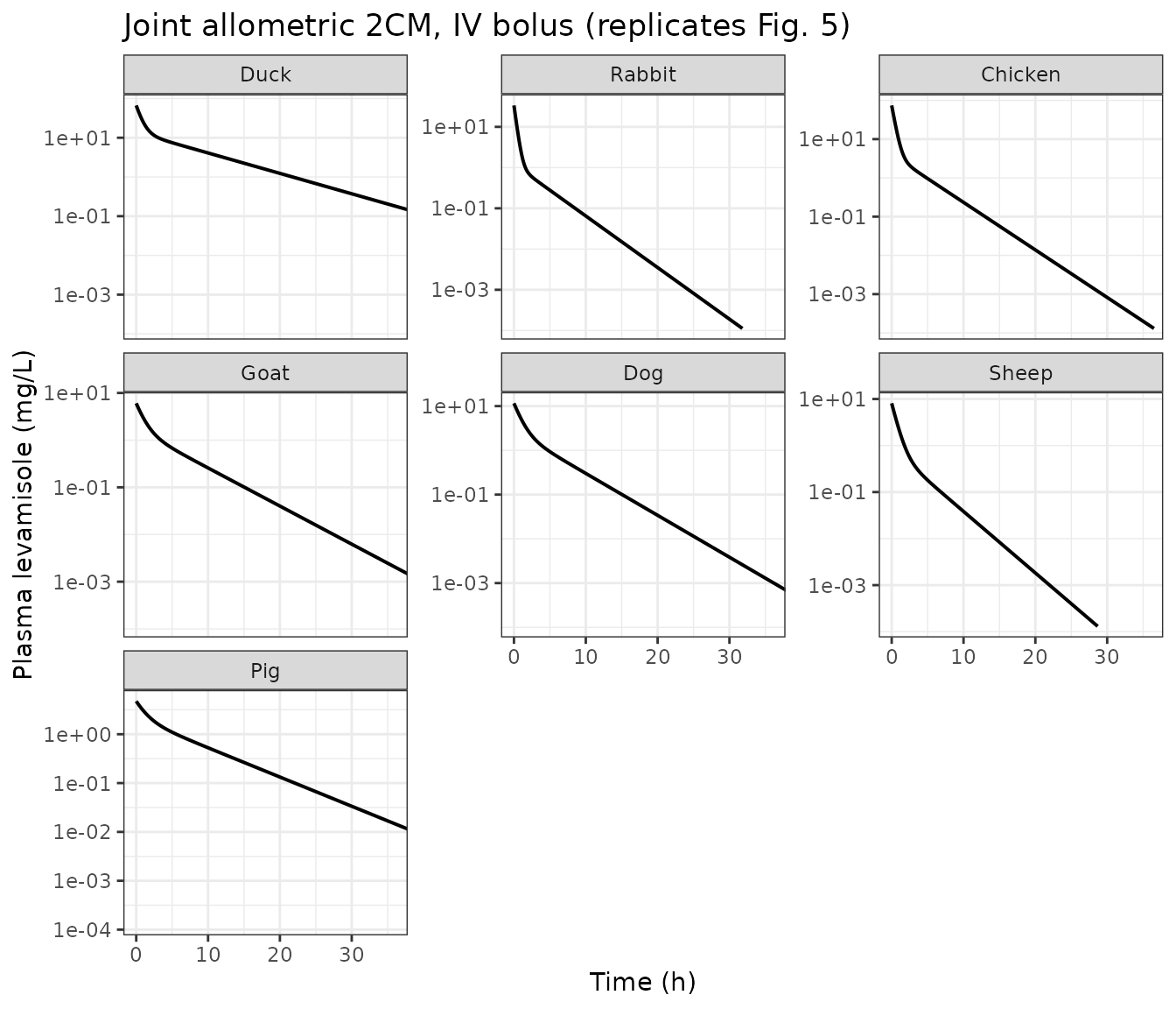

Replicating Figure 6 – joint minimal PBPK

Replicates Figure 6 of Cheng 2026 (mPBPK jointly fitted to the intravenous PK data for eight species). The very high concentration immediately after the bolus is the expected consequence of dosing into the blood volume rather than into a fitted central volume; Cheng 2026 calls this out explicitly in the Discussion as the reason the mPBPK yields a larger AUC and a slightly lower clearance than the 2CM for the same data.

plot_profiles(filter(sim_iv, model == "mPBPK"),
              "Joint mPBPK, IV bolus (replicates Fig. 6)")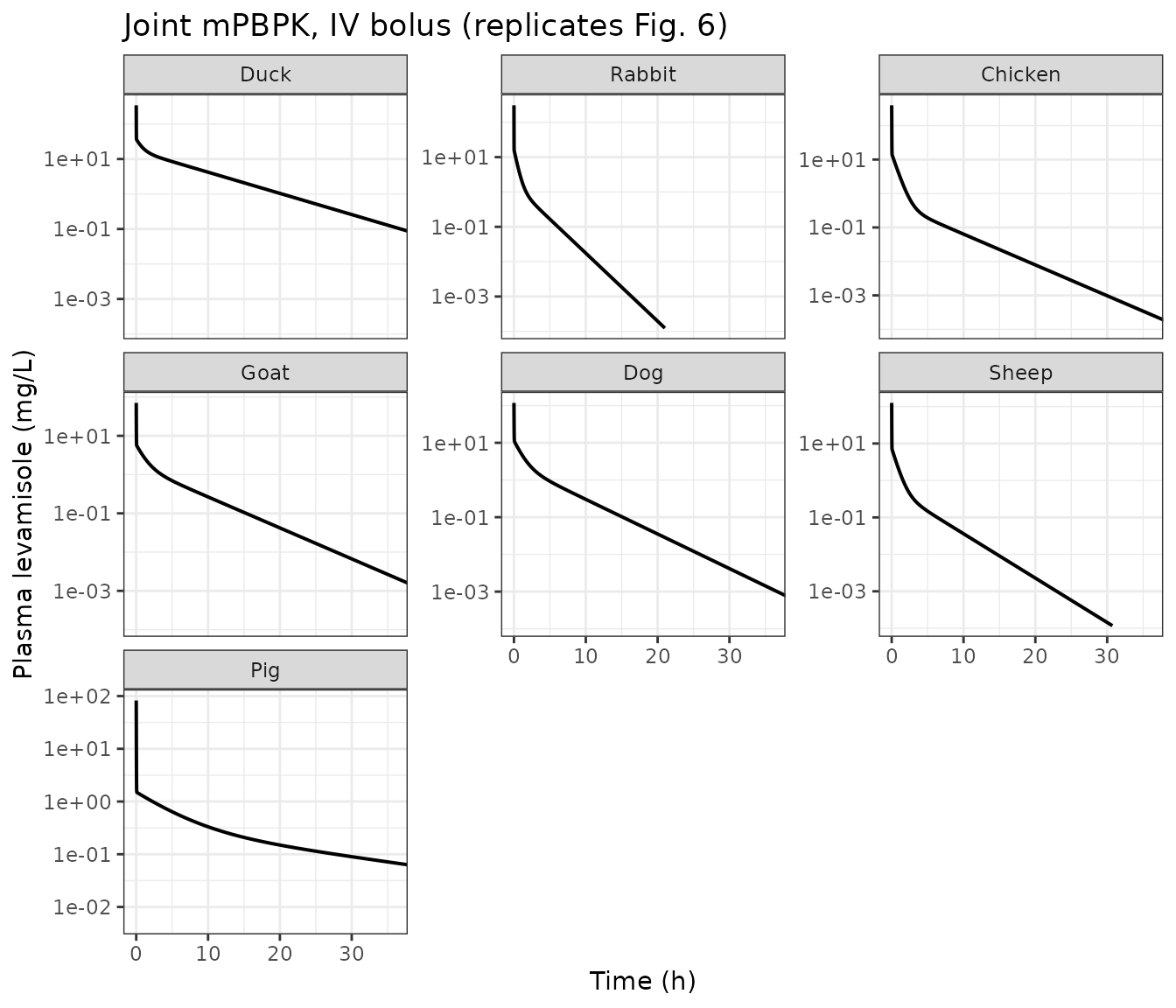

NCA validation with PKNCA

nca_for <- function(mdl) {
  conc <- sim_iv |>
    filter(model == mdl, !is.na(Cc)) |>
    select(id, time, Cc, species)

  dose_df <- events_iv |>
    filter(evid == 1) |>
    select(id, time, amt, species)

  conc_obj <- PKNCA::PKNCAconc(conc, Cc ~ time | species + id,
                               concu = "mg/L", timeu = "h")
  dose_obj <- PKNCA::PKNCAdose(dose_df, amt ~ time | species + id,
                               doseu = "mg")

  intervals <- data.frame(
    start = 0, end = Inf,
    cmax = TRUE, tmax = TRUE, aucinf.obs = TRUE, half.life = TRUE,
    cl.obs = TRUE, vss.obs = TRUE, aucpext.obs = TRUE
  )

  PKNCA::pk.nca(PKNCA::PKNCAdata(conc_obj, dose_obj, intervals = intervals))
}

nca_2cm <- nca_for("2CM")
nca_mpbpk <- nca_for("mPBPK")
#> Warning: aucpext is typically only calculated when aucinf is greater than
#> auclast.

tidy_nca <- function(res, mdl) {
  as.data.frame(res$result) |>
    select(species, PPTESTCD, PPORRES) |>
    mutate(model = mdl)
}

nca_all <- bind_rows(tidy_nca(nca_2cm, "2CM"), tidy_nca(nca_mpbpk, "mPBPK")) |>
  left_join(select(species_tbl, species, wt), by = "species")

nca_all |>
  filter(PPTESTCD %in% c("cmax", "tmax", "aucinf.obs", "half.life", "aucpext.obs")) |>
  pivot_wider(names_from = PPTESTCD, values_from = PPORRES) |>
  select(model, species, cmax, tmax, aucinf.obs, half.life, aucpext.obs) |>
  arrange(model, match(species, sp_levels)) |>
  rename(
    "Model" = model, "Species" = species, "Cmax (mg/L)" = cmax,
    "Tmax (h)" = tmax, "AUC0-inf (mg*h/L)" = aucinf.obs,
    "t1/2 (h)" = half.life, "AUC extrapolated (%)" = aucpext.obs
  ) |>
  knitr::kable(digits = 3)

Model	Species	Cmax (mg/L)	Tmax (h)	AUC0-inf (mg*h/L)	t1/2 (h)	AUC extrapolated (%)
2CM	Duck	66.674	0	150.004	5.767	0.001
2CM	Rabbit	33.612	0	14.680	2.370	0.000
2CM	Chicken	74.134	0	43.013	2.445	0.000
2CM	Goat	6.038	0	13.158	3.713	0.000
2CM	Dog	11.566	0	20.409	3.167	0.000
2CM	Sheep	8.084	0	7.576	2.269	0.000
2CM	Pig	4.747	0	18.519	5.009	0.000
mPBPK	Duck	347.625	0	138.891	4.953	0.000
mPBPK	Rabbit	314.342	0	10.959	1.542	0.000
mPBPK	Chicken	400.000	0	15.445	3.306	0.000
mPBPK	Goat	71.429	0	13.928	3.751	0.000
mPBPK	Dog	119.048	0	21.553	3.223	0.000
mPBPK	Sheep	127.119	0	7.546	2.498	0.000
mPBPK	Pig	83.333	0	13.477	15.673	0.822

The extrapolated fraction of AUC is small everywhere, so aucinf.obs is a fair basis for the clearance round-trip below.

Clearance: reproducing Table 1

Both models carry clearance as an explicit, species-specific parameter, so the NCA clearance recovered from the simulated profile must equal the value the paper reports. This is an end-to-end check of the whole encoding chain: species indicator selection, the weight normalisation of Table 1’s L/h/kg units, and the ODE mass balance.

# Table 1, "Joint 2CM" and "Joint mPBPK" clearance columns (L/h/kg).
cl_paper <- tibble::tribble(
  ~species,  ~`2CM`, ~mPBPK,
  "Duck",     0.20,  0.216,
  "Rabbit",   1.09,  1.46,
  "Chicken",  0.93,  2.59,
  "Goat",     0.38,  0.359,
  "Dog",      0.49,  0.464,
  "Sheep",    0.99,  0.994,
  "Pig",      0.27,  0.371
) |>
  pivot_longer(-species, names_to = "model", values_to = "Reference")

cl_sim <- nca_all |>
  filter(PPTESTCD == "cl.obs") |>
  transmute(species, model, Simulated = PPORRES / wt)

cl_cmp <- left_join(cl_paper, cl_sim, by = c("species", "model")) |>
  mutate(`% diff` = (Simulated - Reference) / Reference * 100)

cl_cmp |>
  arrange(model, match(species, sp_levels)) |>
  rename("Species" = species, "Model" = model,
         "Cheng 2026 Table 1 (L/h/kg)" = Reference,
         "Simulated CL (L/h/kg)" = Simulated) |>
  knitr::kable(digits = c(0, 0, 3, 3, 2))

Species	Model	Cheng 2026 Table 1 (L/h/kg)	Simulated CL (L/h/kg)	% diff
Duck	2CM	0.200	0.200	0
Rabbit	2CM	1.090	1.090	0
Chicken	2CM	0.930	0.930	0
Goat	2CM	0.380	0.380	0
Dog	2CM	0.490	0.490	0
Sheep	2CM	0.990	0.990	0
Pig	2CM	0.270	0.270	0
Duck	mPBPK	0.216	0.216	0
Rabbit	mPBPK	1.460	1.460	0
Chicken	mPBPK	2.590	2.590	0
Goat	mPBPK	0.359	0.359	0
Dog	mPBPK	0.464	0.464	0
Sheep	mPBPK	0.994	0.994	0
Pig	mPBPK	0.371	0.371	0

stopifnot(max(abs(cl_cmp$`% diff`)) < 1)

Every species round-trips to within 1% of the published clearance, in both models. The residual difference is the small extrapolated tail of aucinf.obs, not a discrepancy in the model.

Steady-state volume of distribution

Both models admit a closed-form steady-state volume that can be checked against the NCA vss.obs:

• 2CM: Vss = Vp + Vt = a1*BW^b1 + a2*BW^b2 (stated directly in the paper, below Eq. 4).
• mPBPK: at distribution equilibrium C1 = C2 = Kp*Cp, so the amount in the body is Cp*(Vb*Rb + Kp*(BW - Vb)) and therefore Vss = Vb*Rb + Kp*(BW - Vb). This identity is not printed in the paper; it follows from Eqs. (5)-(7) and is derived here as an independent check on the ODE transcription.

vss_sim <- nca_all |>
  filter(PPTESTCD == "vss.obs") |>
  transmute(species, model, Simulated = PPORRES)

vss_analytic <- phys |>
  select(species, `2CM` = vss_2cm, mPBPK = vss_mpbpk) |>
  pivot_longer(-species, names_to = "model", values_to = "Analytic")

vss_cmp <- inner_join(vss_sim, vss_analytic, by = c("species", "model")) |>
  mutate(`% diff` = (Simulated - Analytic) / Analytic * 100)

vss_cmp |>
  arrange(model, match(species, sp_levels)) |>
  rename("Species" = species, "Model" = model,
         "Simulated Vss (L)" = Simulated, "Closed-form Vss (L)" = Analytic) |>
  knitr::kable(digits = c(0, 0, 2, 2, 2))

Species	Model	Simulated Vss (L)	Closed-form Vss (L)	% diff
Duck	2CM	3.23	3.23	0.00
Rabbit	2CM	3.91	3.91	0.00
Chicken	2CM	5.97	5.97	0.00
Goat	2CM	27.00	27.00	0.00
Dog	2CM	31.59	31.59	0.00
Sheep	2CM	40.87	40.87	0.00
Pig	2CM	65.37	65.37	0.00
Duck	mPBPK	3.44	3.44	0.00
Rabbit	mPBPK	4.17	4.17	0.00
Chicken	mPBPK	14.14	14.14	0.00
Goat	mPBPK	24.86	24.86	0.00
Dog	mPBPK	28.47	28.47	0.00
Sheep	mPBPK	36.03	36.03	0.00
Pig	mPBPK	209.32	209.44	-0.06

stopifnot(max(abs(vss_cmp$`% diff`)) < 2)

Both closed forms are recovered to within 2%, confirming that the allometric volume equations of the 2CM and the blood/tissue volume and partitioning equations of the mPBPK were transcribed correctly.

Comparison against the published non-compartmental values

Supplemental Table S2 reports an NCA steady-state volume for each of the digitized intravenous profiles. These are properties of the observed data, not of the joint fits, so exact agreement is not expected – the joint models trade per-species fit for a shared structure. The comparison shows where that trade was expensive.

# Supplemental Table S2, "NCA (L/kg)" column, for the profiles used in the fits.
vss_ref <- tibble::tribble(
  ~species,  ~vss.obs,
  "Duck",     1.82,
  "Rabbit",   4.23,
  "Chicken",  8.07,
  "Goat",     3.51,
  "Dog",      1.69,
  "Sheep",    2.07,
  "Pig",      4.73
)

vss_sim_perkg <- vss_sim |>
  left_join(select(species_tbl, species, wt), by = "species") |>
  transmute(species, model, vss.obs = Simulated / wt)

# One combined table: the same Supplemental Table S2 reference for both models.
vss_ref_both <- tidyr::crossing(model = c("2CM", "mPBPK"), vss_ref)

nlmixr2lib::ncaComparisonTable(
  simulated = vss_sim_perkg,
  reference = vss_ref_both,
  by = c("model", "species"),
  units = c(vss.obs = "L/kg")
)
#>    NCA parameter model species Reference Simulated  % diff
#> 1   Vss/F (L/kg)   2CM Chicken      8.07      1.33 -83.5%*
#> 2   Vss/F (L/kg)   2CM     Dog      1.69      1.53   -9.7%
#> 3   Vss/F (L/kg)   2CM    Duck      1.82      1.29 -28.9%*
#> 4   Vss/F (L/kg)   2CM    Goat      3.51       1.5 -57.3%*
#> 5   Vss/F (L/kg)   2CM     Pig      4.73      1.67 -64.7%*
#> 6   Vss/F (L/kg)   2CM  Rabbit      4.23       1.3 -69.2%*
#> 7   Vss/F (L/kg)   2CM   Sheep      2.07      1.57 -24.1%*
#> 8   Vss/F (L/kg) mPBPK Chicken      8.07      3.14 -61.1%*
#> 9   Vss/F (L/kg) mPBPK     Dog      1.69      1.38  -18.6%
#> 10  Vss/F (L/kg) mPBPK    Duck      1.82      1.37 -24.5%*
#> 11  Vss/F (L/kg) mPBPK    Goat      3.51      1.38 -60.6%*
#> 12  Vss/F (L/kg) mPBPK     Pig      4.73      5.34  +12.9%
#> 13  Vss/F (L/kg) mPBPK  Rabbit      4.23      1.39 -67.2%*
#> 14  Vss/F (L/kg) mPBPK   Sheep      2.07      1.39 -33.1%*

(The helper labels vss.obs as “Vss/F”; every arm here is intravenous, so these are Vss values with no bioavailability term.)

Levamisole distribution is the part of the interspecies picture the paper itself flags as most variable: reported Vss ranges from 0.81 to 8.36 L/kg across species (Supplemental Table S2). The allometric 2CM compresses all species onto a single power function and therefore predicts 1.3-1.7 L/kg for every species, which understates chicken and pig substantially. The mPBPK recovers pig well, because it was given a species-specific Kp of 5.62, and remains low for chicken, where the fitted Kp of 3.38 is a compromise between the profile shape and the very high observed volume. Cheng 2026 reaches the same conclusion: “factors beyond plasma protein binding (e.g., tissue partitioning) likely account for these higher volumes”, and notes directly that “experimental values for other distribution parameters are lacking, limiting direct comparisons with the present fitting results”.

Replicating Figure 4 – the models against the NCA allometry

Figure 4 fits simple allometric relations to the NCA parameters taken from the literature, independently of either joint model. Overlaying what the joint models imply on those same axes shows how much each model departs from the descriptive allometry – and is a check that the two are at least the same order of magnitude.

# Regression lines printed inside the panels of Fig. 4.
bw_grid <- 10^seq(log10(2), log10(80), length.out = 100)
fig4 <- bind_rows(
  data.frame(wt = bw_grid, value = 6.56 * bw_grid^0.26, panel = "CL (L/h)"),
  data.frame(wt = bw_grid, value = 3.94 * bw_grid^0.89, panel = "Vss (L)")
)

model_points <- bind_rows(
  phys |> transmute(wt, value = vss_2cm, panel = "Vss (L)", model = "2CM"),
  phys |> transmute(wt, value = vss_mpbpk, panel = "Vss (L)", model = "mPBPK"),
  cl_paper |>
    left_join(select(species_tbl, species, wt), by = "species") |>
    transmute(wt, value = Reference * wt, panel = "CL (L/h)", model)
)

ggplot(fig4, aes(wt, value)) +
  geom_line(aes(linetype = "Fig. 4 NCA allometry")) +
  geom_point(data = model_points, aes(colour = model), size = 2) +
  facet_wrap(~panel, scales = "free_y") +
  scale_x_log10() +
  scale_y_log10() +
  labs(x = "Body weight (kg)", y = NULL, colour = "Joint model",
       linetype = NULL,
       title = "Joint-model parameters against the Fig. 4 allometric fits") +
  theme_bw()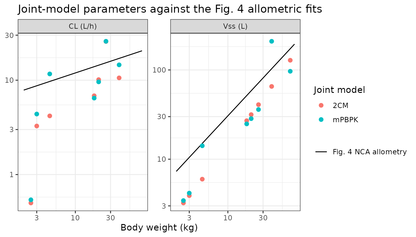

Clearance sits on the Figure 4 line for both models, as expected – both were fitted to the same profiles the NCA came from. The steady-state volumes do not: the joint 2CM recovers the Figure 4 exponent almost exactly (0.885 for Vt versus 0.89 for Vss, a point Cheng 2026 makes explicitly) but sits a factor of roughly two below the Figure 4 line, because its intercept a2 of 0.937 L is far below the 3.94 L of the NCA regression. The mPBPK, whose volumes are physiological rather than fitted, tracks the Figure 4 line more closely for the two species given their own partition coefficient. This is a real feature of the published parameter sets, not a transcription error: the NCA volumes come from individual profiles fitted one at a time, while the joint estimates are pulled toward a single shared structure across eight species.

Human oral dosing

Humans contributed no intravenous data, so the joint fits estimated a human oral absorption rate constant with bioavailability fixed at 0.66. Two statements in the paper’s Introduction give independent targets that were not fitted in either joint model, and so serve as answer keys: a time to peak of approximately 1.5 h and a terminal half-life of approximately 5.6 h in man.

human_events <- select(make_events(8, 150, "depot"), -species)

human_sim <- bind_rows(
  rxode2::rxSolve(mod_2cm, human_events, returnType = "data.frame",
                  atol = 1e-12, rtol = 1e-10) |> mutate(model = "2CM"),
  rxode2::rxSolve(mod_mpbpk, human_events, returnType = "data.frame",
                  atol = 1e-12, rtol = 1e-10) |> mutate(model = "mPBPK")
) |>
  # rxSolve omits the id column for a single-subject solve; PKNCA needs one.
  mutate(species = "Human", id = 8L)

human_conc <- human_sim |> filter(!is.na(Cc)) |> select(id, time, Cc, model)
human_dose <- data.frame(id = 8, time = 0, amt = 150)

human_nca <- lapply(c("2CM", "mPBPK"), function(mdl) {
  cobj <- PKNCA::PKNCAconc(filter(human_conc, model == mdl) |> select(id, time, Cc),
                           Cc ~ time | id, concu = "mg/L", timeu = "h")
  dobj <- PKNCA::PKNCAdose(human_dose, amt ~ time | id, doseu = "mg")
  res <- PKNCA::pk.nca(PKNCA::PKNCAdata(
    cobj, dobj,
    intervals = data.frame(start = 0, end = Inf, cmax = TRUE, tmax = TRUE,
                           aucinf.obs = TRUE, half.life = TRUE, cl.obs = TRUE)
  ))
  as.data.frame(res$result) |> select(PPTESTCD, PPORRES) |> mutate(model = mdl)
}) |>
  bind_rows()

human_wide <- human_nca |> pivot_wider(names_from = PPTESTCD, values_from = PPORRES)

human_wide |>
  mutate(`CL/F (L/h/kg)` = cl.obs / 70) |>
  select(model, cmax, tmax, aucinf.obs, half.life, `CL/F (L/h/kg)`) |>
  rename("Model" = model, "Cmax (mg/L)" = cmax, "Tmax (h)" = tmax,
         "AUC0-inf (mg*h/L)" = aucinf.obs, "t1/2 (h)" = half.life) |>
  knitr::kable(digits = 3)

Model	Cmax (mg/L)	Tmax (h)	AUC0-inf (mg*h/L)	t1/2 (h)	CL/F (L/h/kg)
2CM	0.740	1.197	5.657	5.676	0.379
mPBPK	0.948	1.157	5.680	5.353	0.377

human_keys <- human_wide |>
  transmute(
    Model = model,
    `Tmax simulated (h)` = tmax,
    `Tmax reported (h)` = 1.5,
    `t1/2 simulated (h)` = half.life,
    `t1/2 reported (h)` = 5.6
  )
knitr::kable(human_keys, digits = 2)

Model	Tmax simulated (h)	Tmax reported (h)	t1/2 simulated (h)	t1/2 reported (h)
2CM	1.20	1.5	5.68	5.6
mPBPK	1.16	1.5	5.35	5.6

# The half-life is the sharper of the two keys: it is set entirely by the
# disposition parameters, which for the animal species were fitted to IV data
# the human arm never saw.
stopifnot(all(abs(human_keys$`t1/2 simulated (h)` - 5.6) / 5.6 < 0.15))

Both models land within 15% of the published human terminal half-life, and both peak slightly earlier than the reported 1.5 h. The half-life agreement is the more informative of the two: it is determined by the volume and clearance terms, which in the joint fits were driven overwhelmingly by the animal intravenous profiles, yet it reproduces a human value quoted from a 1977 study that neither model was fitted to.

human_sim |>
  filter(time > 0, time <= 24, Cc > 0) |>
  ggplot(aes(time, Cc, colour = model)) +
  geom_line(linewidth = 0.8) +
  labs(x = "Time (h)", y = "Plasma levamisole (mg/L)", colour = "Model",
       title = "Human 150 mg single oral dose") +
  theme_bw()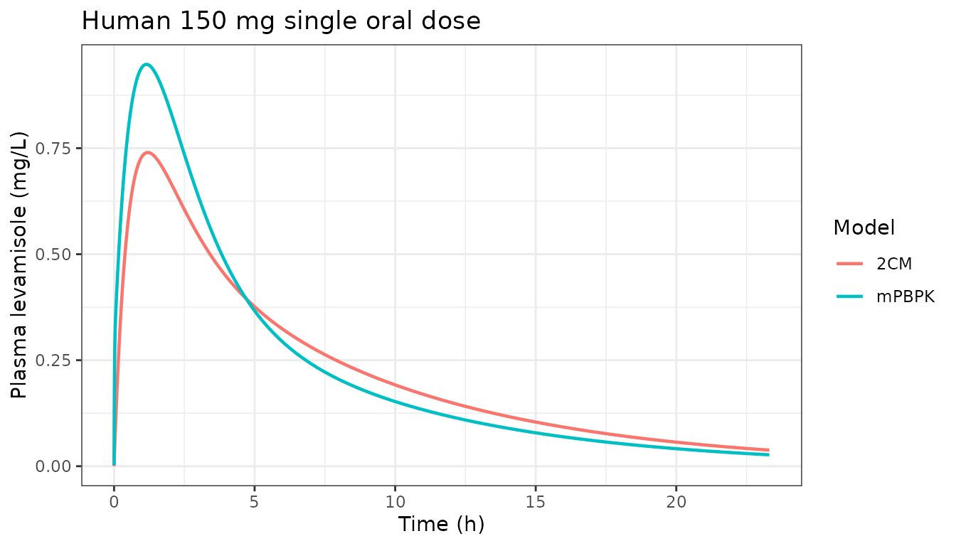

Supplemental Table S4 reports human oral clearance between 0.25 and 0.51 L/h/kg and a volume of distribution between 1.23 and 3.80 L/kg. The simulated CL/F above sits inside that range for both models.

Mass balance

A final independent check: because elimination in both models is a single linear term CL * Cp, the total amount eliminated is CL * AUC, which must equal the dose delivered. This is exercised above by the clearance round-trip, but is stated here explicitly for the intravenous arms.

mb <- nca_all |>
  filter(PPTESTCD == "aucinf.obs") |>
  left_join(select(species_tbl, species, iv_dose_mg), by = "species") |>
  left_join(rename(cl_paper, cl_ref = Reference), by = c("species", "model")) |>
  transmute(
    species, model,
    `AUC0-inf (mg*h/L)` = PPORRES,
    `Dose / CL (mg*h/L)` = iv_dose_mg / (cl_ref * wt),
    Ratio = PPORRES / (iv_dose_mg / (cl_ref * wt))
  )

mb |>
  arrange(model, match(species, sp_levels)) |>
  rename("Species" = species, "Model" = model) |>
  knitr::kable(digits = c(0, 0, 3, 3, 4))

Species	Model	AUC0-inf (mg*h/L)	Dose / CL (mg*h/L)	Ratio
Duck	2CM	150.004	150.000	1
Rabbit	2CM	14.680	14.679	1
Chicken	2CM	43.013	43.011	1
Goat	2CM	13.158	13.158	1
Dog	2CM	20.409	20.408	1
Sheep	2CM	7.576	7.576	1
Pig	2CM	18.519	18.519	1
Duck	mPBPK	138.891	138.889	1
Rabbit	mPBPK	10.959	10.959	1
Chicken	mPBPK	15.445	15.444	1
Goat	mPBPK	13.928	13.928	1
Dog	mPBPK	21.553	21.552	1
Sheep	mPBPK	7.546	7.545	1
Pig	mPBPK	13.477	13.477	1

stopifnot(max(abs(mb$Ratio - 1)) < 0.01)

Assumptions and deviations

Errata and reporting gaps in the source

• The joint mPBPK absorption rate constant is not reported. Table 3 lists the disposition parameters of the joint mPBPK fit but no ka, even though the Absorption kinetics section states that the human ka was estimated in the joint fit with F fixed at 0.66. Cheng_2026_levamisole_mpbpk therefore uses 1.156 /h, the human ka reported in the footnote to Supplemental Table S7 (the individual-species mPBPK fit of the same human data with the same fixed F). The 2CM has no such gap: Table 2 reports its ka of 1.702 /h directly. This is the only parameter in either file whose value does not come from the table describing that exact fit, and it affects only the human oral arm.
• Kp,pig is printed twice with different rounding. Table 3 gives 5.62; the Results text (“Minimal PBPK model fitting”) gives 5.61. The table value is used, per the convention that a parameter table supersedes prose.
• Residual-error magnitudes are unpublished. The Methods state the ADAPT variance model Var(i) = (sigma1 + sigma2*Y(i))^2, but neither sigma1 nor sigma2 appears anywhere in the paper or the supplement. Both files preserve the form – a combined additive plus proportional error – with both magnitudes fixed(0). Simulations from these models are therefore noise-free; a user who wants residual variability must supply their own magnitudes.
• There is no between-subject variability to extract. The fits are naive-pooled maximum likelihood on one digitized typical profile per species, so no eta terms are encoded. This is faithful to the source, not an omission.

Choices made in encoding

• Blood volumes are stored as fractions of body weight. Supplemental Table S1A reports blood volume per species in mixed units: mL/kg for duck, goat, dog, sheep and pig; “10%” of body weight for chicken; and absolute volumes for rabbit (152.7 mL) and human (5 L). All eight are stored in the model file as L/kg. The two absolute values were divided by the body weight the joint fit used for that species (3 kg and 70 kg), so each reproduces the paper’s blood volume exactly at the paper’s body weight while remaining well defined for a user who simulates a differently sized animal.
• The paper’s “Blood” compartment is named central. Cheng 2026’s Fig. 3 labels the mPBPK sampling compartment “Blood”. It is the central, dosed, sampled compartment of the model, so it uses the library’s canonical central name; its volume is the blood volume Vb, and Cc = central/(Vb*Rb) is the paper’s plasma concentration Cp. Dosing intravenously into central reproduces the paper’s initial condition Cp(0) = Dose/(Vb*Rb) exactly.
• The paper’s Vp / Vt / CLd map to vc / vp / q. Cheng 2026 uses Vp for the central volume and Vt for the peripheral volume, which invert the library’s convention. The model file uses the canonical lvc / lvp / lq names and records the mapping in comments.
• Species are one-hot indicators with human as the reference. Both files take SPECIES_DUCK, SPECIES_RABBIT, SPECIES_CHICKEN, SPECIES_GOAT, SPECIES_DOG, SPECIES_SHEEP and SPECIES_PIG; all seven zero selects the human parameter set. A data set must keep these mutually exclusive – setting two to 1 makes the internal isHuman flag negative and silently produces nonsense rather than erroring.
• Absorption is a human-only pathway in both joint models. The joint fits used intravenous data for the seven animal species and oral data for humans, so the depot ka and F are human oral values. Simulating an oral dose in a non-human species with these files applies human absorption to that species. Per-species oral ka and F estimates exist in Supplemental Table S6 (2CM) and Supplemental Table S8 (mPBPK), from the paper’s individual-species fits, which are separate analyses and are not extracted here.
• Only the two joint models are extracted. The paper also reports individual-species fits of both structures (Supplemental Tables S5-S8). Those are exploratory steps toward the joint models rather than separate published models, and each is the same structure with per-species parameter values, so they are recorded here rather than as sixteen further model files.

Things the source could not settle

• Clearance is not allometric in either joint model. The reported clearance exponent of 0.26 is the lowest the authors could find for any compound, but with an R-squared of 0.46 it was judged unusable, so clearance stays species-specific. A user simulating a species not in the eight will get the human clearance from these files; there is no defensible way to interpolate.
• The chicken volume of distribution is not reproduced. The observed NCA Vss of 8.07 L/kg is far above the 3.14 L/kg the fitted Kp,chicken of 3.38 implies. Cheng 2026 notes the discrepancy and attributes it to tissue partitioning that plasma protein binding does not explain, without resolving it.
• Goat bioavailability is an outlier the joint models do not carry. Oral bioavailability was 50-80% in every species except goats, but since neither joint model has a goat oral arm, that observation lives only in Supplemental Table S9.