Risperidone in beagle dogs (Chen 2019)
Source:vignettes/articles/Chen_2019_risperidone_dog.Rmd
Chen_2019_risperidone_dog.RmdModel and source
- Citation: Chen F, Liu H, Wang B, Yang L, Cai W, Jiao Z, Yang Z, Chen Y, Quan Y, Xiang X, Wang H. (2020). Physiologically Based Pharmacokinetic Modeling to Understand the Absorption of Risperidone Orodispersible Film. Front Pharmacol 10:1692. doi:10.3389/fphar.2019.01692.
- Description: Preclinical (beagle dog). Three-compartment intravenous disposition model for risperidone, fitted by the authors to the mean plasma profile after a 1 mg intravenous bolus in four beagle dogs (DAS 2.0) and used unaltered as the disposition layer of their GastroPlus ACAT/OCCAT absorption model for a risperidone orodispersible film. Disposition-only: the oral / supralingual / sublingual absorption was simulated in GastroPlus and is not reproduced here. Typical-value model (no IIV or residual error reported).
- Article: https://doi.org/10.3389/fphar.2019.01692 (open access, PMC7008171)
Chen et al. built a GastroPlus 9.7 absorption model (ACAT for the gastrointestinal tract linked to OCCAT for the oral cavity) for a 1 mg risperidone orodispersible film (ODF) in beagle dogs. Its disposition layer is an empirical three-compartment model the authors fitted to their own intravenous data in DAS 2.0 and entered in GastroPlus “without further alteration” (Methods, Model Development). That three-compartment model is what this package carries. The ACAT/OCCAT absorption is proprietary platform code driven by physicochemical inputs (Table 2: log P, pKa, solubility, Peff = 5.3894e-4 cm/s, Fu-t = 0.15382, 51% first-pass extraction) and is not reproduced.
Population
Four healthy beagle dogs (2 male, 2 female) weighing 9.04 +/- 1.88 kg, fasted 12 h, received 1 mg risperidone in a four-period crossover with a 1-week washout: i.v. solution, i.g. dissolved ODF, supralingual ODF and sublingual ODF (Methods, Pharmacokinetic Study). Plasma was sampled to 32 h and assayed by HPLC-MS/MS (LLOQ 0.2 ng/mL). Only the i.v. period informs the disposition model; GastroPlus was given the cohort mean weight of 9.0425 kg (Table 2).
Source trace
| Quantity | Value | Source |
|---|---|---|
lcl |
CL = 0.5903 L/h/kg | Table 2, Disposition parameters |
lvc |
Vc = 0.3139 L/kg | Table 2 |
lk12 |
K12 = 16.352 1/h | Table 2 |
lk21 |
K21 = 9.007 1/h | Table 2 |
lk13 |
K13 = 0.4625 1/h | Table 2 |
lk31 |
K31 = 0.4103 1/h | Table 2 |
| V2, V3 (derived, not parameters) | 0.56988, 0.35383 L/kg | Table 2; equal vc*k12/k21, vc*k13/k31
|
| Terminal t1/2 (check) | 2.43 h | Table 2 |
| Body weight scaling | linear per kg, 9.0425 kg fitted | Table 2 (‘Body weight’) |
| Three-compartment structure | empirical 3-cmt, i.v. | Methods, Model Development |
propSd |
fixed(0) | not reported (fit to the mean profile) |
| Observed i.v. NCA | AUC, Cmax, CL, t1/2 | Table 1 |
Internal consistency of Table 2
Table 2 prints both the rate constants and the peripheral volumes, plus a terminal half-life. The volumes follow from the rate constants, and the half-life is the slowest eigenvalue of the rate matrix; both are exact checks of the transcription that need no simulation.
wt <- 9.0425
vc <- 0.3139
kel <- 0.5903 / vc
k12 <- 16.352
k21 <- 9.007
k13 <- 0.4625
k31 <- 0.4103
K <- matrix(
  c(-(kel + k12 + k13), k21, k31,
    k12, -k21, 0,
    k13, 0, -k31),
  nrow = 3, byrow = TRUE
)
lambda <- sort(-eigen(K)$values)
closed <- tibble::tibble(
  quantity = c("V2 (L/kg)", "V3 (L/kg)", "Terminal t1/2 (h)"),
  model = c(vc * k12 / k21, vc * k13 / k31, log(2) / lambda[1]),
  table2 = c(0.56988, 0.35383, 2.43)
) |>
  mutate(pct_diff = 100 * (model - table2) / table2)
knitr::kable(closed, digits = 4)| quantity | model | table2 | pct_diff |
|---|---|---|---|
| V2 (L/kg) | 0.5699 | 0.5699 | -0.0003 |
| V3 (L/kg) | 0.3538 | 0.3538 | 0.0016 |
| Terminal t1/2 (h) | 2.4269 | 2.4300 | -0.1285 |
The half-lives of the three phases are 2.43, 0.767, 0.0257 h.
Simulation
A 1 mg i.v. bolus to the typical 9.0425 kg dog, on the paper’s sampling schedule (plus a 2-minute sample: Table 1 reports the i.v. Tmax as 0.03 h) and a dense grid for plotting. A 200-dog weight cohort drawn from the reported 9.04 +/- 1.88 kg shows the spread that weight alone produces under the per-kg scaling.
mod <- readModelDb("Chen_2019_risperidone_dog")

paper_times <- c(0.0333, 0.167, 0.333, 0.5, 0.75, 1, 1.5, 2, 3, 4, 6, 8, 12, 24, 32)
obs_times <- sort(unique(c(0, paper_times, seq(0, 32, by = 0.1))))

ev_typ <- rxode2::et(amt = 1, cmt = "central") |>
  rxode2::et(obs_times, cmt = "central") |>
  as.data.frame() |>
  mutate(id = 1L, WT = 9.0425, treatment = "i.v. 1 mg")

sim_typ <- rxode2::rxSolve(mod, ev_typ, keep = c("WT", "treatment")) |>
  as.data.frame()

set.seed(2019)
n_cohort <- 200
wts <- pmax(rnorm(n_cohort, 9.04, 1.88), 5)
ev_coh <- lapply(seq_len(n_cohort), function(i) {
  mutate(ev_typ, id = i, WT = wts[i])
}) |>
  bind_rows()
sim_coh <- rxode2::rxSolve(mod, ev_coh, keep = c("WT", "treatment")) |>
  as.data.frame()
#> Warning: multi-subject simulation without without 'omega'
Replicate Figure 3A (i.v. arm)
Figure 3A of Chen 2019 plots the mean +/- SD i.v. profile. The figure itself is not digitised here; the published Table 1 i.v. Cmax (214.97 ng/mL at 0.03 h) is overlaid as the one observed point the paper tabulates.
band <- sim_coh |>
  filter(time > 0) |>
  group_by(time) |>
  summarise(lo = quantile(Cc, 0.05), hi = quantile(Cc, 0.95), .groups = "drop")

ggplot() +
  geom_ribbon(data = band, aes(time, ymin = lo, ymax = hi), alpha = 0.25) +
  geom_line(data = filter(sim_typ, time > 0), aes(time, Cc)) +
  geom_point(aes(x = 0.03, y = 214.97), shape = 15, size = 2.5) +
  geom_hline(yintercept = 0.2, linetype = "dotted") +
  scale_y_log10() +
  labs(x = "Time after dose (h)", y = "Risperidone plasma concentration (ng/mL)")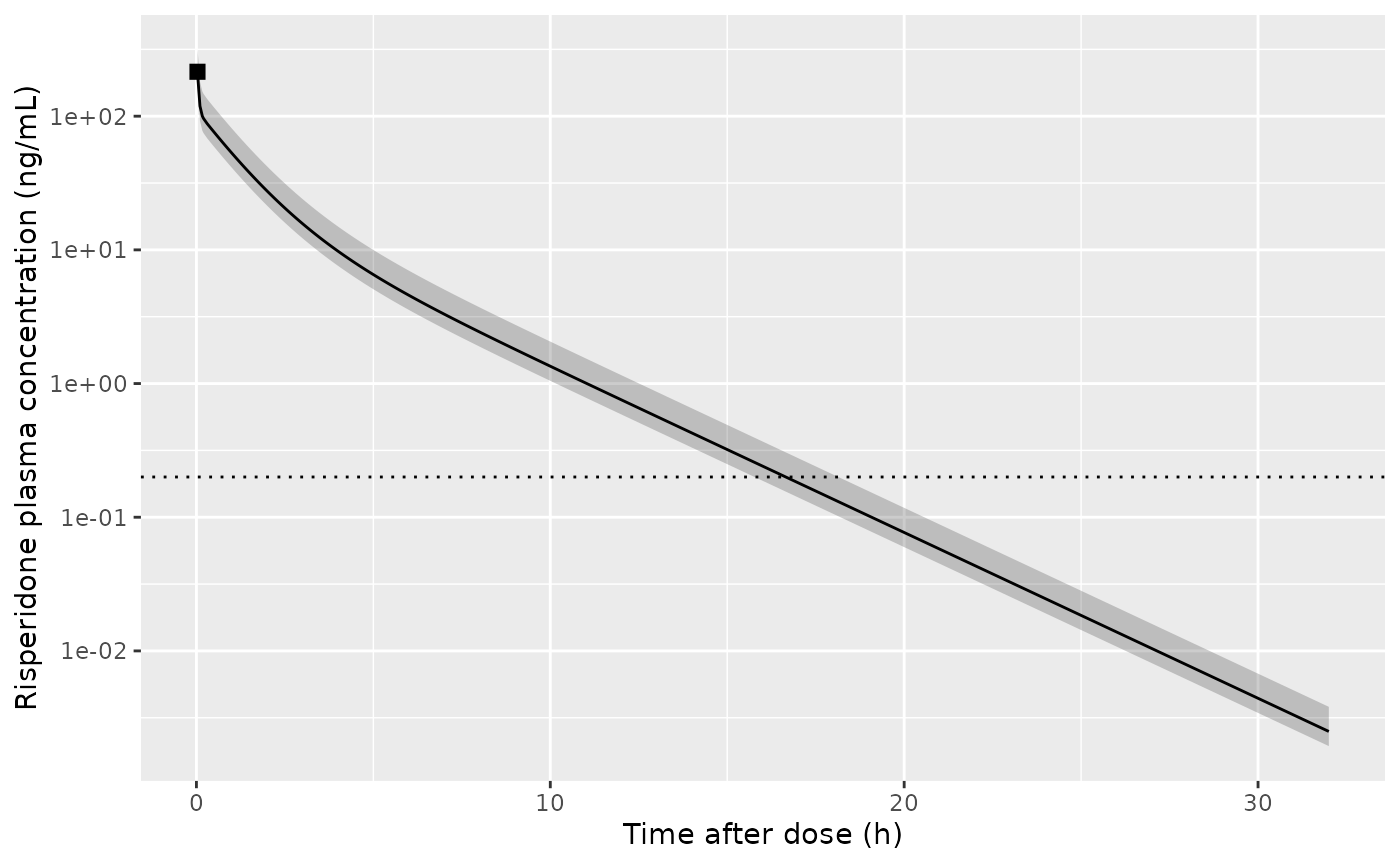
Replicates the i.v. arm of Figure 3A of Chen 2019: typical dog (line), 5th-95th percentile of a 200-dog weight cohort (band), Table 1 observed Cmax (point). Dotted line: LLOQ 0.2 ng/mL.
PKNCA validation
NCA on the typical-dog profile at the paper’s sampling times, censored at the 0.2 ng/mL LLOQ as the observed data were, with the pre-dose blank at time 0 and the first sample at 2 minutes. The dose is given to PKNCA in ug so that clearance comes out in L/h.
conc_df <- sim_typ |>
  filter(time %in% c(0, paper_times)) |>
  # rxode2 returns the time-0 row after the bolus (C0 = dose / Vc); the study
  # drew a blank pre-dose sample instead, so time 0 is set to 0 as in Table 1.
  mutate(
    Cc = ifelse(time == 0, 0, Cc),
    Cc = ifelse(time > 0 & Cc < 0.2, NA_real_, Cc),
    id = 1L
  ) |>
  filter(!is.na(Cc)) |>
  select(id, time, Cc, treatment)

dose_df <- tibble::tibble(id = 1L, time = 0, amt_ug = 1000, treatment = "i.v. 1 mg")

conc_obj <- PKNCA::PKNCAconc(conc_df, Cc ~ time | treatment + id)
dose_obj <- PKNCA::PKNCAdose(dose_df, amt_ug ~ time | treatment + id, route = "intravascular")
intervals <- data.frame(
  start = 0, end = Inf,
  cmax = TRUE, tmax = TRUE, auclast = TRUE, aucinf.obs = TRUE,
  half.life = TRUE, cl.obs = TRUE
)
nca_res <- PKNCA::pk.nca(PKNCA::PKNCAdata(conc_obj, dose_obj, intervals = intervals))
nca_tab <- as.data.frame(nca_res$result) |>
  select(PPTESTCD, PPORRES)
knitr::kable(nca_tab, digits = 3)| PPTESTCD | PPORRES |
|---|---|
| auclast | 182.292 |
| cmax | 206.546 |
| tmax | 0.033 |
| tlast | 12.000 |
| clast.obs | 0.757 |
| lambda.z | 0.299 |
| r.squared | 1.000 |
| adj.r.squared | 0.999 |
| lambda.z.time.first | 6.000 |
| lambda.z.time.last | 12.000 |
| lambda.z.n.points | 3.000 |
| clast.pred | 0.752 |
| half.life | 2.320 |
| span.ratio | 2.586 |
| aucinf.obs | 184.827 |
| cl.obs | 5.410 |
Comparison against published NCA
published <- tibble::tibble(
  treatment = "i.v. 1 mg",
  cmax = 214.97,
  auclast = 177.02,
  aucinf.obs = 179.10,
  half.life = 1.37,
  cl.obs = 7.69
)
cmp_nca <- nlmixr2lib::ncaComparisonTable(
  simulated = nca_res,
  reference = published,
  by = "treatment",
  params = c("cmax", "auclast", "aucinf.obs", "half.life", "cl.obs"),
  units = c(
    cmax = "ng/mL", auclast = "ng*h/mL", aucinf.obs = "ng*h/mL",
    half.life = "h", cl.obs = "L/h"
  ),
  tolerance_pct = 20
)
knitr::kable(cmp_nca, caption = "Simulated typical dog vs. Table 1 of Chen 2019 (i.v., mean of n = 4). * differs from reference by >20%.")| NCA parameter | treatment | Reference | Simulated | % diff |
|---|---|---|---|---|
| Cmax (ng/mL) | i.v. 1 mg | 215 | 207 | -3.9% |
| AUC0-∞ (obs) (ng*h/mL) | i.v. 1 mg | 179 | 185 | +3.2% |
| AUClast (ng*h/mL) | i.v. 1 mg | 177 | 182 | +3.0% |
| t½ (h) | i.v. 1 mg | 1.37 | 2.32 | +69.3%* |
| CL/F (L/h) | i.v. 1 mg | 7.69 | 5.41 | -29.6%* |
attr(cmp_nca, "footnote")
#> [1] "* differs from reference by more than ±20%."

nca_val <- setNames(nca_tab$PPORRES, nca_tab$PPTESTCD)
stopifnot(
  abs(nca_val[["aucinf.obs"]] / 179.10 - 1) < 0.10,
  abs(nca_val[["cmax"]] / 214.97 - 1) < 0.10
)
AUC and Cmax agree within 5%. The two starred rows are not model discrepancies:
- CL. Table 1 reports the arithmetic mean of the four individual clearances (7.69 L/h). Dose over the mean AUC is 1000 / 179.10 = 5.58 L/h, within 3.1% of the model. A mean of individual ratios exceeds the ratio of means whenever AUC varies between animals, and here the i.v. AUC SD was 113 of 179.
- t1/2. Table 1’s 1.37 h is the mean of individual NCA half-lives from DAS, whereas Table 2 prints the model’s own terminal half-life as 2.43 h, which the eigenvalue check above reproduces exactly. The two numbers disagree inside the paper itself; the model follows Table 2.
Assumptions and deviations
- Disposition only. The oral (i.g.), supralingual and sublingual arms were simulated in GastroPlus ACAT/OCCAT, whose transit, dissolution (Z-factor) and oral-mucosa equations are platform code not printed in the paper. No first-order absorption rate was reported, and none is invented here. The observed relative bioavailability of the ODF was 57-65% (Table 1) and the GastroPlus first-pass extraction 51% (Table 2), for users building an absorption layer.
-
Per-kg scaling. Table 2 reports CL and volumes per
kg; they are scaled linearly by
WT, as GastroPlus applies them. The paper fitted a single mean profile, so weight scaling was not estimated. -
No variability. No IIV or residual error was
reported (a DAS fit to pooled i.v. data).
propSdisfixed(0); the cohort band above reflects weight only. - Year. The article is in Front Pharmacol volume 10 (2019, DOI year 2019) but was published online 3 February 2020; the file stem uses 2019.
- Metabolite. 9-OH risperidone was measured (Figure 3B) but not modelled.