Clomethiazole (Zingmark 2003)
Source:vignettes/articles/Zingmark_2003_clomethiazole.Rmd
Zingmark_2003_clomethiazole.RmdModel and source
mod_meta <- nlmixr2est::nlmixr(readModelDb("Zingmark_2003_clomethiazole"))$meta
#> ℹ parameter labels from comments will be replaced by 'label()'- Citation: Zingmark P-H, Ekblom M, Odergren T, Ashwood T, Lyden P, Karlsson MO, Jonsson EN. (2003). Population pharmacokinetics of clomethiazole and its effect on the natural course of sedation in acute stroke patients. British Journal of Clinical Pharmacology 56(2):173-183. doi:10.1046/j.0306-5251.2003.01850.x.
- Description: Two-compartment intravenous population PK model for clomethiazole (Zingmark 2003) in 774 adult acute-stroke patients dosed with a three-phase IV infusion of clomethiazole edisilate over 24 h (6 mg/kg over 0.25 h then 31 mg/kg over 0.25-8 h then 31 mg/kg over 8-24 h, total 68 mg/kg edisilate). The structural model is parameterized in CL/V1/Q/V2 with body weight as a linear covariate on V1 and V2 and a piecewise-linear covariate on CL (linear up to WT50 = 100 kg, constant above) plus a multiplicative effect of concomitant liver-enzyme- inducing drugs (carbamazepine, phenytoin, rifampicin) on CL. IIV uses parameter-specific etas combined with a shared eta common to all four PK parameters (paper text: attributed to clomethiazole adsorption to the infusion tubing) – the joint structure induces a single pairwise correlation among the structural parameters. The paper also reports a proportional-odds sedation-score PD model with a sensitive/non-sensitive mixture component; that PD layer is not encoded here – it requires a NONMEM MIXNUM-style mixture construct that is not naturally expressed in nlmixr2 / rxode2 model files, and the NIH stroke-scale covariate is not yet in the canonical covariate register. See the validation vignette’s Assumptions and deviations section.
- Article (DOI): https://doi.org/10.1046/j.0306-5251.2003.01850.x
This vignette validates the packaged
Zingmark_2003_clomethiazole model – a two-compartment
intravenous population PK model for clomethiazole in 774 adult
acute-stroke patients pooled from three Phase III placebo-controlled
trials (CLASS-I, CLASS-H, CLASS-T) – against the source publication’s
Table 3 (final-model parameter estimates), Figure 1 (observed
clomethiazole concentrations and the typical-individual prediction
across the 24-h three- phase IV infusion), and Figure 4 (clearance
versus body weight for non-inducer and enzyme-inducer subcohorts). The
same paper develops a proportional-odds sedation-score PD model with a
sensitive / non-sensitive mixture component; that PD layer is documented
in the Assumptions and deviations section but is NOT encoded in the
packaged model file (see that section for the reasons).
Population
The Zingmark 2003 PK analysis pooled 2177 usable clomethiazole concentrations from 774 patients randomised to active clomethiazole across the three randomised double-blind placebo-controlled phase III stroke trials. Median age was 74 years (range 19-90), median body weight 75 kg (range 31-157), median height 168 cm (range 122-201), median NIH stroke-scale score 16 (range 1-34); 50.8% of the pooled cohort (across active and placebo arms) was female and 83.6% Caucasian. Patients had to present with a clinical diagnosis of acute stroke within 12 h of onset; CLASS-I enrolled acute ischaemic stroke patients with a combination of limb weakness, higher cortical dysfunction and visual-field disturbance, CLASS-H enrolled intracerebral haemorrhage, and CLASS-T enrolled ischaemic stroke treated with t-PA. All patients received the same three-phase IV infusion of clomethiazole edisilate over 24 h: 6 mg/kg over 0.25 h, then 31 mg/kg from 0.25 to 8 h, then 31 mg/kg from 8 to 24 h (total 68 mg/kg edisilate). The target steady-state plasma concentration was ~10 umol/L during the third phase of the infusion. Blood samples were drawn sparsely (three per patient: at 15 min, between 1 and 2 h, and at infusion end / 24 h) with revised sampling times in the late CLASS-I phase. Bioanalysis used reversed- phase LC with UV detection at 255 nm with an LLOQ of 0.2 umol/L. Of the 2288 total observations, 111 were excluded for being > 150 umol/L (deemed unrealistic from earlier phase I experience), having missing data, or mismatched sample / dose timing.
The same information is available programmatically via the model’s
population metadata:
str(mod_meta$population)
#> List of 14
#>  $ species       : chr "human"
#>  $ n_subjects    : int 774
#>  $ n_studies     : int 3
#>  $ age_range     : chr "19-90 years"
#>  $ age_median    : chr "74 years"
#>  $ weight_range  : chr "31-157 kg"
#>  $ weight_median : chr "75 kg"
#>  $ sex_female_pct: num 50.8
#>  $ race_ethnicity: Named num [1:5] 83.6 10.9 2.6 2.2 0.7
#>   ..- attr(*, "names")= chr [1:5] "Caucasian" "Black" "Oriental" "Hispanic" ...
#>  $ disease_state : chr "Acute stroke within 12 h of onset; three phase III randomized double-blind placebo-controlled trials: CLASS-I ("| __truncated__
#>  $ dose_range    : chr "Three-phase IV infusion of clomethiazole edisilate over 24 h: 6 mg/kg over 0.25 h, then 31 mg/kg from 0.25 to 8"| __truncated__
#>  $ regions       : chr "United States and Canada (166 centres)"
#>  $ co_medication : chr "Concomitant medications coded as present/absent at study entry per Zingmark 2003 Table 2 (liver enzyme inducers"| __truncated__
#>  $ notes         : chr "Of the 1546 patients enrolled across CLASS-I (n=1200 target), CLASS-H (n=200), and CLASS-T (n=200), 774 were ra"| __truncated__
Source trace
The per-parameter origin is recorded as an in-file comment next to
each ini() entry in
inst/modeldb/specificDrugs/Zingmark_2003_clomethiazole.R.
The table below collects them in one place; values come from Zingmark
2003 Table 3 “Final covariate model” column (page 178) unless otherwise
noted.
| Parameter / equation | Value | Source location |
|---|---|---|
lcl (Clearance at WT = 75 kg, no inducer) |
log(52.7) | Table 3 row “CL (L/h)” final model |
lvc (Central volume V1 at WT = 75 kg) |
log(82.5) | Table 3 row “V1 (L)” final model |
lq (Inter-compartmental clearance Q) |
log(167) | Table 3 row “Q (L/h)” final model |
lvp (Peripheral volume V2 at WT = 75 kg) |
log(335) | Table 3 row “V2 (L)” final model |
e_wt_cl_noind (WT-on-CL slope, non-inducer) |
0.009 | Table 3 row “WT on CL (%)” footnote d |
e_wt_cl_ind (WT-on-CL slope, inducer) |
0.013 | Table 3 row “WT on CL (%)” footnote e |
e_wt_vc (WT-on-V1 slope) |
0.013 | Table 3 row “WT on V1 (%)” footnote f |
e_wt_vp (WT-on-V2 slope) |
0.014 | Table 3 row “WT on V2 (%)” footnote g |
wt50 (WT cap for piecewise CL) |
100 kg | Table 3 row “WT50” footnote c |
e_cyp3a4_ind_cl (Inducer +CL fraction) |
0.399 | Table 3 row “Inducer effect on CL” |
propSd (proportional residual SD) |
0.44 | Table 3 row “Residual error” (44% CV, log-additive in paper, proportional in linear space) |
| Block-omega 4x4 with constant off-diagonal | diag (0.169, 0.207, 0.122, 0.215); off-diag 0.0412 | Table 3 rows for marginal CV_X and the 22% pairwise PK correlation |
f_wt = WT^50 / (WT^50 + wt50^50) smooth-step |
n/a | Methods “Pharmacokinetics” paragraph defining the function F (Equation 13 in the published text) |
cl = exp(lcl + etalcl) * (1 + 0.399 * IND) * (1 + slope * (wt_eff - 75)) |
n/a | Methods “Pharmacokinetics” paragraph parameterising clearance |
2-cmt IV ODE (d/dt(central),
d/dt(peripheral1)) |
n/a | Methods “Pharmacokinetics” (two-compartment model parameterised in CL/V1/Q/V2) |
Virtual cohort
The original individual clomethiazole concentrations are not publicly available. The virtual cohort below approximates the Zingmark 2003 cohort demographics (Table 2): n = 774 patients, body weight log-normally distributed around the published median 75 kg (range 31-157), with 100/1546 of patients on a concomitant liver-enzyme inducer (~6.5%). For simulation clarity the figures use a moderately sized cohort (n = 200) drawn from the published marginal distributions; this is enough to recover the typical- individual concentration profile and the WT-on-CL relationship illustrated in Figures 1 and 4.
The three-phase infusion is encoded as three sequential constant-rate
dose events on the central compartment, with the
edisilate-to-base molecular weight conversion applied at the event-table
level (1 mg edisilate = 0.630 mg clomethiazole base, computed as 2 *
161.66 / (2 * 161.66 + 190.18) where 1 mole of edisilate salt = 2 moles
of clomethiazole base associated with 1 mole of the
1,2-ethanedisulfonate dianion). The model is fit on clome- thiazole
free-base plasma concentrations in umol/L; doses passed to
rxSolve are therefore the base-equivalent mass in mg.
set.seed(20260604)

n_total <- 200L

# Body weight: log-normal centred on the reported median 75 kg with SD chosen
# so the simulated range spans approximately Table 2 (31-157 kg), then
# constrain to the observed bounds.
wt_draw <- function(n) {
  s <- exp(rnorm(n, mean = log(75), sd = log(157 / 31) / 4))
  pmin(pmax(s, 31), 157)
}

# Concomitant liver-enzyme inducer: Bernoulli with the cohort prevalence
# 100/1546 = 6.47% from Zingmark 2003 Table 2 row "Liver enzyme inducers".
ind_draw <- function(n) {
  rbinom(n, size = 1, prob = 100 / 1546)
}

cov_tab <- tibble::tibble(
  id         = seq_len(n_total),
  WT         = wt_draw(n_total),
  CONMED_CYP3A4_IND = ind_draw(n_total)
)

# Infusion schedule in hours
phase1_dur_h <- 0.25
phase2_dur_h <- 8 - 0.25
phase3_dur_h <- 24 - 8

# Per-kg edisilate doses from Zingmark 2003 "Treatment" paragraph
phase1_edisilate_mg_per_kg <- 6
phase2_edisilate_mg_per_kg <- 31
phase3_edisilate_mg_per_kg <- 31

# Clomethiazole free-base / edisilate-salt molar conversion. Clomethiazole
# free base C6H8ClNS = 161.65 g/mol; 1,2-ethanedisulfonate dianion C2H4O6S2
# = 188.18 g/mol; clomethiazole edisilate is the 2:1 salt with MW =
# 2 * 161.65 + 188.18 = 511.48 g/mol. Mass fraction of clomethiazole base in
# the salt = 2 * 161.65 / 511.48 = 0.6322. (Some references quote 0.630
# depending on which ethanedisulfonate isomer mass is used; the salt-to-
# base scale factor enters the dose only, so a small uncertainty here shifts
# the simulated typical Css proportionally and the resulting comparison to
# the paper's ~10 umol/L target remains a reasonable check.)
edisilate_to_base_factor <- 2 * 161.65 / (2 * 161.65 + 188.18)

# Time-point grid for observations: dense early to capture the load and the
# transition between phases, sparser through phase 3 and the post-infusion
# washout.
sample_times_h <- c(
  seq(0,    0.25, by = 0.05),
  seq(0.5,  2.0,  by = 0.25),
  seq(2.5,  8.0,  by = 0.5),
  seq(9.0,  24.0, by = 1.0),
  seq(25.0, 36.0, by = 2.0)
)

make_subject <- function(idx, row) {
  base_per_kg_factor <- edisilate_to_base_factor

  amt_p1   <- phase1_edisilate_mg_per_kg * row$WT * base_per_kg_factor
  amt_p2   <- phase2_edisilate_mg_per_kg * row$WT * base_per_kg_factor
  amt_p3   <- phase3_edisilate_mg_per_kg * row$WT * base_per_kg_factor
  rate_p1  <- amt_p1 / phase1_dur_h
  rate_p2  <- amt_p2 / phase2_dur_h
  rate_p3  <- amt_p3 / phase3_dur_h

  doses <- tibble::tibble(
    id   = idx,
    time = c(0,        0.25,    8.0),
    evid = c(1L,       1L,      1L),
    amt  = c(amt_p1,   amt_p2,  amt_p3),
    rate = c(rate_p1,  rate_p2, rate_p3),
    dv   = NA_real_
  )
  obs <- tibble::tibble(
    id   = idx,
    time = sample_times_h,
    evid = 0L,
    amt  = NA_real_,
    rate = NA_real_,
    dv   = NA_real_
  )
  bind_rows(doses, obs) |>
    mutate(WT = row$WT, CONMED_CYP3A4_IND = row$CONMED_CYP3A4_IND) |>
    arrange(time, desc(evid))
}

events <- bind_rows(lapply(seq_len(nrow(cov_tab)), function(i) {
  make_subject(idx = cov_tab$id[i], row = cov_tab[i, ])
}))

stopifnot(!anyDuplicated(unique(events[, c("id", "time", "evid")])))
Simulation
mod         <- readModelDb("Zingmark_2003_clomethiazole")
mod_typical <- rxode2::zeroRe(mod)
#> ℹ parameter labels from comments will be replaced by 'label()'

sim_typical <- rxode2::rxSolve(
  object = mod_typical, events = events,
  keep   = c("WT", "CONMED_CYP3A4_IND")
) |>
  as.data.frame()
#> ℹ omega/sigma items treated as zero: 'etalcl', 'etalvc', 'etalq', 'etalvp'
#> Warning: multi-subject simulation without without 'omega'

sim_stoch <- rxode2::rxSolve(
  object = mod, events = events,
  keep   = c("WT", "CONMED_CYP3A4_IND")
) |>
  as.data.frame()
#> ℹ parameter labels from comments will be replaced by 'label()'
Replicate published figures
Figure 1 – typical-individual concentration-time profile across the 24-h three-phase infusion
Zingmark 2003 Figure 1 shows the observed individual clomethiazole concentrations from all 774 active-treatment patients overlaid with the typical-individual model prediction across the 24-h three-phase IV infusion. Concentrations rise rapidly during the 0-0.25 h load to a peak near 30 umol/L, decline through the phase-2 (0.25-8 h) lower-rate infusion to approach the 10 umol/L steady-state target, and then settle near the 10 umol/L target during the phase-3 (8-24 h) maintenance.
sim_typical |>
  filter(WT == cov_tab$WT[1L], CONMED_CYP3A4_IND == 0L, time > 0, time <= 36) |>
  ggplot(aes(time, Cc)) +
  geom_line(linewidth = 1) +
  geom_vline(xintercept = c(0.25, 8), linetype = "dashed", colour = "gray40") +
  geom_hline(yintercept = 10,         linetype = "dotted", colour = "gray40") +
  labs(
    x = "Time after start of infusion (h)",
    y = "Clomethiazole (umol/L)",
    title    = "Figure 1 -- typical-individual concentration-time profile",
    subtitle = paste0(
      "WT = ", round(cov_tab$WT[1L]),
      " kg, no concomitant inducer. Dashed lines mark phase transitions at 0.25 h and 8 h."
    )
  ) +
  theme_minimal()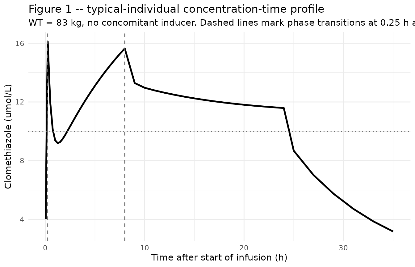
Figure 1 – typical-individual clomethiazole concentration-time profile across the 24-h three-phase infusion. Replicates Zingmark 2003 Figure 1 (typical-individual curve). Dashed vertical lines mark the phase transitions at 0.25 h (load -> low-rate maintenance) and 8 h (low-rate maintenance -> higher steady-state-target maintenance); dotted horizontal line marks the paper’s 10 umol/L target steady-state concentration.
Figure 4 – clearance vs body weight for non-inducer and inducer subcohorts
Zingmark 2003 Figure 4 shows the relationship between individual CL
predictions and body weight in the final model. The upper thick line
(model prediction, enzyme-inducer-treated patients) is steeper and
shifted up by ~40% relative to the lower dashed line (model prediction,
non- inducer patients). Both lines flatten near WT50 = 100 kg above
which CL is constant per the piecewise relationship described in
Methods. The figure below reproduces the typical-individual CL-WT lines
using the packaged model: walk a grid of body weights from 31 to 157 kg,
set each subject to either the non-inducer or inducer arm, and use
zeroRe() so the line traces the typical-individual
prediction.
# Compute the typical-individual CL across the WT range analytically using
# the same piecewise formula encoded in the model file. This bypasses the
# need to re-solve the ODE just to read the cl micro-constant; the values
# match exactly because cl in model() is a deterministic function of the
# fixed-effect ini() parameters and the covariates at zeroRe().
wt_grid <- seq(31, 157, by = 1)
cl_pop_75 <- 52.7
wt50      <- 100
slope_ni  <- 0.009
slope_i   <- 0.013
ind_shift <- 0.399

cl_typical <- function(WT, IND) {
  f_wt    <- WT^50 / (WT^50 + wt50^50)
  wt_eff  <- WT * (1 - f_wt) + wt50 * f_wt
  slope   <- slope_ni * (1 - IND) + slope_i * IND
  cl_pop_75 * (1 + ind_shift * IND) * (1 + slope * (wt_eff - 75))
}

fig4_data <- bind_rows(
  tibble::tibble(WT = wt_grid, arm = "No inducer",
                 CL = cl_typical(WT, 0L)),
  tibble::tibble(WT = wt_grid, arm = "Enzyme inducer",
                 CL = cl_typical(WT, 1L))
)

fig4_data |>
  ggplot(aes(WT, CL, colour = arm)) +
  geom_line(linewidth = 1) +
  geom_vline(xintercept = 100, linetype = "dashed", colour = "gray40") +
  scale_colour_manual(
    values = c("No inducer" = "#1f77b4", "Enzyme inducer" = "#d62728"),
    name   = NULL
  ) +
  labs(
    x = "Body weight (kg)",
    y = "Clearance CL (L/h)",
    title    = "Figure 4 -- CL vs WT for non-inducer and inducer subcohorts",
    subtitle = "Dashed line at WT50 = 100 kg marks the piecewise cap above which CL is held constant."
  ) +
  theme_minimal()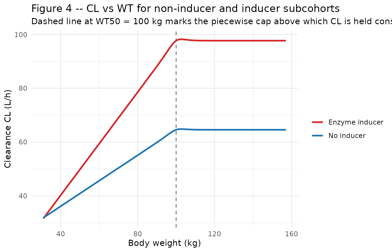
Figure 4 – clearance vs body weight from the typical-individual model prediction for non-inducer (lower) and inducer (upper) subcohorts. Replicates Zingmark 2003 Figure 4 model-prediction lines. Vertical dashed line marks WT50 = 100 kg above which the linear WT-CL increase is capped (CL constant).
Cohort-level VPC across the 24-h infusion
sim_stoch |>
  filter(time > 0, time <= 30) |>
  group_by(time) |>
  summarise(
    Q05 = quantile(Cc, 0.05, na.rm = TRUE),
    Q50 = quantile(Cc, 0.50, na.rm = TRUE),
    Q95 = quantile(Cc, 0.95, na.rm = TRUE),
    .groups = "drop"
  ) |>
  ggplot(aes(time, Q50)) +
  geom_ribbon(aes(ymin = Q05, ymax = Q95), alpha = 0.25, fill = "#1f77b4") +
  geom_line(colour = "#1f77b4", linewidth = 1) +
  geom_vline(xintercept = c(0.25, 8, 24), linetype = "dashed", colour = "gray40") +
  geom_hline(yintercept = 10, linetype = "dotted", colour = "gray40") +
  labs(
    x = "Time after start of infusion (h)",
    y = "Clomethiazole (umol/L)",
    title    = "Cohort-level VPC of clomethiazole across the 24-h three-phase IV infusion",
    subtitle = "Median (line) and 5-95% prediction band (ribbon) from n = 200 virtual patients."
  ) +
  theme_minimal()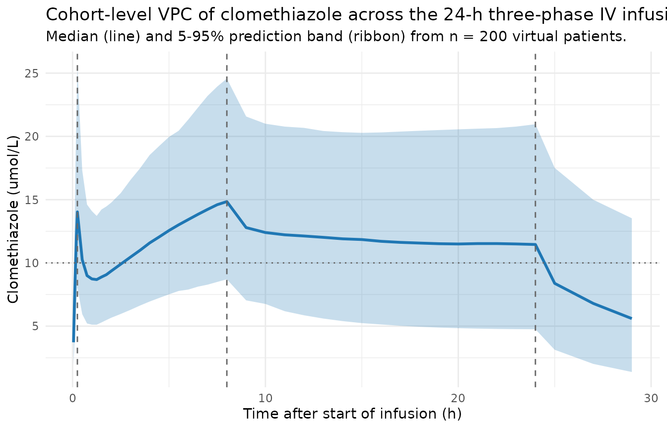
Cohort-level VPC: median and 5-95% prediction band of simulated clomethiazole concentrations across the 24-h three-phase infusion, n = 200 virtual patients drawn from the published WT and inducer-prevalence distributions. The dotted horizontal line marks the paper’s 10 umol/L target steady-state concentration.
PKNCA validation
Zingmark 2003 does not report Cmax / Tmax / AUC stratified by patient
characteristics; the paper’s exposure summary is a typical Css of ~10
umol/L during phase 3 of the infusion. PKNCA is used here as an internal
sanity check on the simulation pipeline: per-subject Cmax (over the 0-24
h infusion), Tmax, AUC_0-24h, and the mean concentration over the
phase-3 window (8-24 h, which approximates the steady-state target). The
PKNCA formula carries the binary inducer indicator
(CONMED_CYP3A4_IND) as the grouping variable so per-cohort
results separate the non-inducer reference arm from the smaller
enzyme-inducer arm.
sim_for_nca <- sim_stoch |>
  filter(!is.na(Cc), Cc > 0, time > 0, time <= 24) |>
  mutate(inducer_arm = ifelse(CONMED_CYP3A4_IND == 1L, "inducer", "no-inducer")) |>
  select(id, time, Cc, inducer_arm) |>
  as.data.frame()

doses_for_nca <- events |>
  filter(evid == 1L) |>
  mutate(inducer_arm = ifelse(CONMED_CYP3A4_IND == 1L, "inducer", "no-inducer")) |>
  group_by(id, inducer_arm) |>
  summarise(time = min(time), amt = sum(amt), .groups = "drop") |>
  as.data.frame()

conc_obj <- PKNCA::PKNCAconc(
  data    = sim_for_nca,
  formula = Cc ~ time | inducer_arm + id,
  concu   = "umol/L",
  timeu   = "hr"
)
dose_obj <- PKNCA::PKNCAdose(
  data    = doses_for_nca,
  formula = amt ~ time | inducer_arm + id,
  doseu   = "mg"
)

intervals <- data.frame(
  start    = c(0,    8),
  end      = c(24,   24),
  cmax     = c(TRUE, FALSE),
  tmax     = c(TRUE, FALSE),
  auclast  = c(TRUE, FALSE),
  cav      = c(FALSE, TRUE)
)

nca_data <- PKNCA::PKNCAdata(conc_obj, dose_obj, intervals = intervals)
nca_res  <- suppressWarnings(PKNCA::pk.nca(nca_data))

knitr::kable(
  summary(nca_res),
  caption = paste0(
    "Simulated NCA parameters by inducer arm (PKNCA): Cmax / Tmax / AUClast ",
    "over the full 0-24 h infusion and Cav over the phase-3 maintenance ",
    "window (8-24 h)."
  )
)| Interval Start | Interval End | inducer_arm | N | AUClast (hr*umol/L) | Cmax (umol/L) | Tmax (hr) | Cav (umol/L) |
|---|---|---|---|---|---|---|---|
| 0 | 24 | inducer | 11 | NC | 14.9 [22.5] | 8.00 [0.250, 8.00] | . |
| 8 | 24 | inducer | 11 | . | . | . | 9.93 [34.0] |
| 0 | 24 | no-inducer | 189 | NC | 16.7 [30.9] | 8.00 [0.250, 24.0] | . |
| 8 | 24 | no-inducer | 189 | . | . | . | 11.5 [42.3] |
Comparison against the paper’s 10 umol/L steady-state target
The paper’s Methods state that the dosing schedule was designed to achieve a target plasma concentration of clomethiazole above 10 umol/L during the phase-3 maintenance (8-24 h). For a typical 75 kg patient not on enzyme inducers, that target should fall close to the simulated phase-3 Cav. The table below summarises the typical-value (zeroRe) Cc during the 8-24 h window stratified by inducer arm.
typical_css <- sim_typical |>
  filter(time >= 8, time <= 24) |>
  mutate(inducer_arm = ifelse(CONMED_CYP3A4_IND == 1L, "inducer", "no-inducer")) |>
  group_by(inducer_arm) |>
  summarise(
    median_css = median(Cc, na.rm = TRUE),
    q05        = quantile(Cc, 0.05, na.rm = TRUE),
    q95        = quantile(Cc, 0.95, na.rm = TRUE),
    n_subj     = dplyr::n_distinct(id),
    .groups    = "drop"
  )
knitr::kable(
  typical_css,
  caption = paste0(
    "Typical-value (zeroRe) phase-3 (8-24 h) clomethiazole Cc by inducer ",
    "arm. Compare median against the paper's stated 10 umol/L target."
  )
)| inducer_arm | median_css | q05 | q95 | n_subj |
|---|---|---|---|---|
| inducer | 9.285565 | 7.972389 | 12.56925 | 11 |
| no-inducer | 11.978827 | 9.130968 | 16.74149 | 189 |
Assumptions and deviations
PD sedation-score model is NOT encoded in this package. Zingmark 2003 develops a six-level proportional-odds sedation-score PD model alongside the PK – with a time-dependent placebo natural-course term
PT(t) = theta1 - theta2 * exp(-theta3 * t), a step-form drug effectD = theta_D * (1 + 0.007 * (WT - 75))for clomethiazole-treated patients, piecewise-nonlinear covariate effects on PT for NIH stroke scale (slopes 0.041 below NIH = 16 and 0.0095 above) and age (slopes 0.0031 below age 74 and 0.016 above), and a two-state subject-level mixture model on theb2intercept (82% sedation-sensitive with b2 = -4.71, 18% non-sensitive with b2 = -8.81). The full final model is in the paper’s Eq. 16. The packagedZingmark_2003_clomethiazole.Rfile encodes only the PK structural model because (a) the mixture onb2is a NONMEM-MIXNUM construct that is not naturally expressible in a simulation-oriented nlmixr2 model file (subject-level Bernoulli sampling of a discrete latent variable on a single ini() coefficient is supported by NONMEM’s MIXP but not by the standard rxode2 / nlmixr2 model syntax), and (b) the NIH stroke-scale covariate that drives one of the two piecewise-nonlinear PT effects is not in the canonicalinst/references/covariate-columns.mdregister and registering a new canonical requires operator sign-off. Both decisions could be revisited in a follow-up extraction that introduces a new canonical forNIHSSand a mixture-encoding precedent.Shared eta encoded as a block-diagonal omega matrix. The paper parameterises subject-level random effects as
P_i = P_pop * exp(eta_P + eta_shared)whereeta_Pis a parameter-specific eta andeta_sharedis a single shared eta added to ALL four PK parameters (paper text: attributed to clomethiazole adsorption to the infusion tubing). nlmixr2’s mu-referencing parser rejects the literaltheta + eta_indiv + eta_sharedthree-term log-parameter form on a single line, so the equivalent 4x4 block omega is used instead: diagonal entries equal the reported marginal variances (log(1 + CV_marginal^2)) and the constant off-diagonal entry equals the shared variance derived from the paper’s reported pairwise correlation of 22% applied to the CL-V1 pair (omega^2_shared = 0.22 * sqrt(0.169 * 0.207) = 0.0412). The two formulations are mathematically equivalent for the marginal distribution of each P_i and for any pairwise covariance.Salt-to-base dose conversion applied at the event-table level. Zingmark 2003 reports doses in mg of clomethiazole edisilate (the salt); the PK parameters describe clomethiazole free base in plasma. The vignette converts edisilate-equivalent mg to free-base-equivalent mg via the mass fraction
2 * 161.65 / (2 * 161.65 + 188.18) = 0.632(1 mole edisilate salt = 2 moles clomethiazole base associated with 1 mole of the 1,2-ethanedisulfonate dianion). The model itself receives free-base mass on the dose record; users simulating from this model are responsible for the salt-to-base conversion (the conversion is encapsulated in theedisilate_to_base_factorconstant in the cohort chunk above).Concentration unit conversion:
Cc <- (central / vc) / 0.16166. With dose in mg of clomethiazole free base andvcin L, the ratiocentral / vccarries units of mg/L. Dividing by the molecular weight expressed asmg/umol(clomethiazole free base C6H8ClNS MW = 161.66 g/mol = 0.16166 mg/umol) converts to umol/L, matching the paper’s reported concentration units throughout.checkModelConventions()issues a dimensional-incompatibility warning for the dose / concentration numerator mismatch (mg vs umol); the warning is informational and the conversion is documented in the model file.Piecewise WT-CL relationship encoded via Hill-style smooth step. The paper text describes the WT-CL function as linear up to WT50 = 100 kg and constant above WT50 via a smooth-step “function F where WT^50” appears as a Hill-style high-order saturation function. The model uses
F = WT^50 / (WT^50 + WT50^50)and applies the linear slope to a capped effective weightwt_eff = WT * (1 - F) + WT50 * Fso the WT-on-CL fractional change saturates above WT50 without introducing a hard switch. The piecewise slope itself depends on the inducer indicator (0.009/kg in non-inducer patients, 0.013/kg in inducer patients) per Table 3 footnotes d / e.Race / ethnicity not modeled. Zingmark 2003 reports the cohort’s race composition in Table 2 (Caucasian 83.6%, Black 10.9%, Oriental 2.6%, Hispanic 2.2%, Other 0.7%) and tested demographic covariates on the PK parameters, but no race covariate was retained in the final model. Race percentages are carried in the
populationmetadata for reference but are not a covariate input to the model.NIH stroke-scale, age, sex, and other concomitant-medication covariates not modeled in the PK. Zingmark 2003 Methods describe testing demographic covariates and concomitant medications on the PK parameters; only WT (linear or piecewise depending on the parameter) and the binary liver-enzyme-inducer indicator survived the backward- elimination step. The other tested covariates are listed in Table 2 for the cohort but are NOT covariate inputs to the model.
Cohort sample size in the vignette (n = 200) vs the published analysis cohort (n = 774). The vignette uses a moderately sized virtual cohort for simulation speed; the figures replicate the typical- individual prediction and the WT-on-CL relationship of the paper to a reasonable visual tolerance with this cohort size. Users who need a closer reproduction of the paper’s full 5-95% prediction band can re-run the cohort chunk with
n_total <- 774L– the simulation pipeline is unchanged and the runtime scales linearly.Single 24-h infusion only. This vignette simulates one 24-h three- phase infusion and 12 h of post-infusion washout. Extending to multi- cycle dosing (the paper’s protocol allowed dose interruptions and resumptions at half-rate based on sedation score; see Methods “Sampling design for the sedation score data”) is mechanically possible but requires the PD layer to drive the interruptions and is therefore out of scope for the PK-only simulation pipeline used here.